import sys
import subprocess

sys.path.append(
    subprocess.check_output(["grass", "--config", "python_path"], text=True).strip()
)

import grass.script as gs
import grass.jupyter as gj
from grass.tools import Tools

session = gj.init("~/grassdata/nc_spm_08_grass7/PERMANENT")
tools = Tools()

tools.g_region(vector="zipcodes_wake")Basic Vector Data Analysis with GRASS
vector
beginner
intermediate
Python
Learn the core vector operations in GRASS: exploring attributes, selecting by attribute and by location, buffering, overlay, and counting features per area.
Introduction
Vector data represents geographic features as points, lines, and areas, each linked to a table of attributes. GRASS has a large family of v.* tools for working with them. This tutorial introduces the operations you will reach for most often, using a single worked example: analyzing how schools in Wake County, North Carolina relate to major roads and administrative areas.
Along the way we will:
- explore a vector map and its attribute table,
- select by attribute with v.extract,
- buffer features with v.buffer,
- select by location with v.select,
- perform spatial operations with v.overlay, and
- count features per area with v.vect.stats.
NoteDemo dataset
This tutorial uses the standard GRASS North Carolina sample dataset (nc_spm_08_grass7), which includes schools_wake (points), roadsmajor (lines), and zipcodes_wake (areas).
NoteHow to run this tutorial
The code uses the GRASS Python API in a Jupyter notebook. If you are new to running GRASS from Python, see the Get started with GRASS & Python tutorial. Every step also works from the GRASS GUI or command line; just use the tool name (for example v.buffer) with the same parameters.
Setup and exploration
Start a GRASS session and set the computational region to the extent of the ZIP code areas, which cover the whole county. For vector-only work the region mainly controls what the maps display.
NoteGRASS version
The examples use the grass.tools API (the Tools class), introduced in GRASS 8.5. On earlier versions you can run the same tools with gs.run_command("v.buffer", ...).
Before analyzing a layer, it helps to know what it contains. v.info reports the feature types and counts, and its -c flag lists the attribute columns.
# Feature summary (points, lines, areas ...)
print(tools.v_info(map="schools_wake", flags="t").text)

# Attribute columns
print(tools.v_info(map="schools_wake", flags="c").text)
schools_wake has 167 point features. Let’s look at the attribute table itself. v.db.select can return the table as JSON, which pandas turns into a tidy table:
import pandas as pd

pd.DataFrame(
    tools.v_db_select(
        map="schools_wake",
        columns="NAMESHORT,GLEVEL,ADDRCITY,CORECAPACI",
        format="json",
    )["records"]
).head()| NAMESHORT | GLEVEL | ADDRCITY | CORECAPACI |
|---|---|---|---|
| SWIFT CREEK | E | Raleigh | 448.0 |
| BRIARCLIFF | E | Cary | 540.0 |
| FARMINGTON WOODS | E | Cary | 523.0 |
| CARY | H | Cary | 2287.0 |
| ADAMS | E | Cary | 722.0 |
The GLEVEL column records each school’s level (E for elementary, M for middle, H for high, and so on), which we use next to select schools by attribute. Let’s first draw an overview map: the ZIP code areas, the major roads, and the schools. In grass.jupyter, a Map object collects display layers and renders them together.
overview = gj.Map(width=500)
overview.d_vect(map="zipcodes_wake", type="area",
                fill_color="235:235:235", color="180:180:180")
overview.d_vect(map="roadsmajor", color="90:90:90", width=1)
overview.d_vect(map="schools_wake", icon="basic/circle", size=7,
                fill_color="200:30:30", color="white")
overview.d_barscale(flags="n", at=(58, 9), bgcolor="white")
overview.show()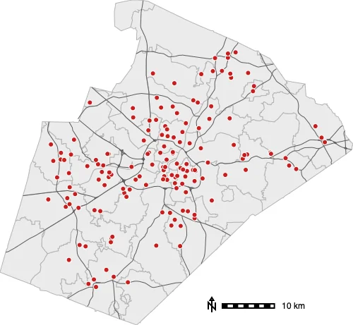
Selecting by attribute
To keep just the elementary schools (GLEVEL='E'), use v.extract with a SQL where clause.
tools.v_extract(input="schools_wake", output="elementary", where="GLEVEL='E'")
print(tools.v_info(map="elementary", flags="t").text)  # points=95
attr_map = gj.Map(width=500)
attr_map.d_vect(map="zipcodes_wake", type="area",
fill_color="235:235:235", color="180:180:180")
attr_map.d_vect(map="roadsmajor", color="90:90:90", width=1)
attr_map.d_vect(map="schools_wake", icon="basic/circle", size=6,
fill_color="180:180:180", color="none")
attr_map.d_vect(map="elementary", icon="basic/circle", size=8,
fill_color="30:120:200", color="white")
attr_map.d_barscale(flags="n", at=(58, 9), bgcolor="white")
attr_map.show()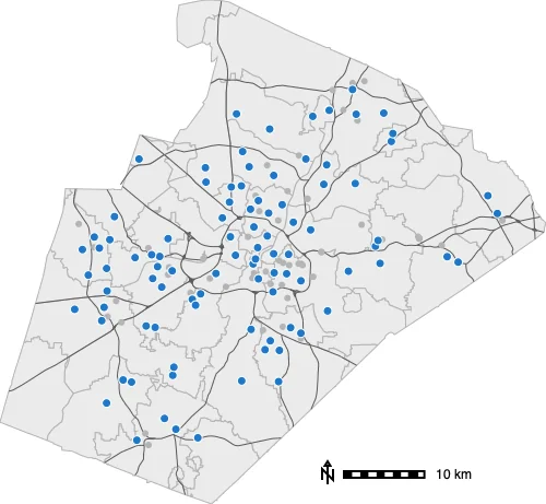
Buffering
A buffer is an area of a given radius around features. Here we buffer the major roads by 500 m with v.buffer to represent an “along a major road” corridor. The result is an area map.
tools.v_buffer(input="roadsmajor", output="road_buffer", distance=500)buffer_map = gj.Map(width=500)
buffer_map.d_vect(map="zipcodes_wake", type="area",
fill_color="235:235:235", color="180:180:180")
buffer_map.d_vect(map="road_buffer", type="area", fill_color="255:200:120", color="none")
buffer_map.d_vect(map="roadsmajor", color="120:70:20", width=1)
buffer_map.d_barscale(flags="n", at=(58, 9), bgcolor="white")
buffer_map.show()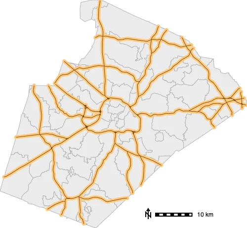
Selecting by location
Now we combine two layers spatially: v.select keeps features of one map based on their spatial relationship to another. With operator=overlap, we keep the elementary schools that fall inside the road buffer.
tools.v_select(ainput="elementary", binput="road_buffer",
               output="schools_near", operator="overlap")
print(tools.v_info(map="schools_near", flags="t").text)  # points=15
Only 15 out of the 95 elementary schools lie within 500 m of a major road, a reminder that major roads here are highways, while most schools sit on local streets.
near_map = gj.Map(width=500)
near_map.d_vect(map="zipcodes_wake", type="area",
                fill_color="235:235:235", color="180:180:180")
near_map.d_vect(map="road_buffer", type="area", fill_color="255:230:200", color="none")
near_map.d_vect(map="roadsmajor", color="150:110:60", width=1)
near_map.d_vect(map="elementary", icon="basic/circle", size=7,
                fill_color="150:150:150", color="none")
near_map.d_vect(map="schools_near", icon="basic/circle", size=9,
                fill_color="20:150:60", color="white")
near_map.d_barscale(flags="n", at=(58, 9), bgcolor="white")
near_map.show()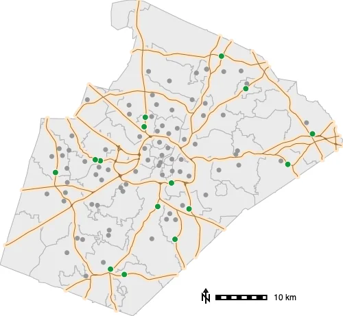
Overlaying layers
v.overlay combines two area maps with set operations. With operator=and we get the intersection, the part of the road corridor that falls within each ZIP code area. The output keeps the attributes of both inputs (prefixed a_ and b_).
tools.v_overlay(ainput="road_buffer", binput="zipcodes_wake",
                operator="and", output="buffer_by_zip")
overlay_map = gj.Map(width=500)
overlay_map.d_vect(map="zipcodes_wake", type="area",
fill_color="235:235:235", color="180:180:180")
overlay_map.d_vect(map="buffer_by_zip", type="area",
fill_color="120:180:220", color="80:80:80", width=1)
overlay_map.d_barscale(flags="n", at=(58, 9), bgcolor="white")
overlay_map.show()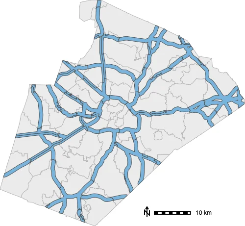
Because each piece now carries its ZIP code, we can measure how much of each ZIP code is within reach of a major road. v.to.db computes the area of every polygon, and a grouped SQL query with db.select sums it per ZIP code:
tools.v_to_db(map="buffer_by_zip", option="area", columns="reach_area", units="kilometers")

# db.select also returns JSON, so the same pandas pattern works here
pd.DataFrame(
    tools.db_select(
        sql="SELECT b_ZIPNAME, ROUND(SUM(reach_area), 1) AS reach_km2 "
            "FROM buffer_by_zip GROUP BY b_ZIPNAME ORDER BY reach_km2 DESC",
        format="json",
    )["records"]
).head(6)| b_ZIPNAME | reach_km2 |
|---|---|
| RALEIGH | 158.3 |
| WAKE FOREST | 59.1 |
| ZEBULON | 42.0 |
| GARNER | 33.4 |
| CARY | 32.2 |
| APEX | 29.5 |
Raleigh leads by a wide margin because it is the largest ZIP code and is crossed by the most major roads.
Counting features per area
A common summary is “how many points fall in each area?” v.vect.stats counts the points of one map within the areas of another and writes the result to the area map’s attribute table. We first create a copy of the ZIP codes map with g.copy so the original is untouched.
tools.g_copy(vector=("zipcodes_wake", "zip_counts"))
tools.v_vect_stats(points="schools_wake", areas="zip_counts", count_column="n_schools")
Each ZIP code now has an n_schools value (ranging from 0 to 17 here). We map it as a choropleth with d.vect.thematic, using quantile classes so each color holds a similar number of areas.
choropleth = gj.Map(width=500)
choropleth.d_vect_thematic(
    map="zip_counts", column="n_schools", algorithm="qua", nclasses=5,
    colors="255:245:215,255:200:120,240:140:60,200:70:30,140:20:20",
)
choropleth.d_vect(map="roadsmajor", color="120:120:120", width=1)
choropleth.d_barscale(flags="n", at=(58, 9), bgcolor="white")
choropleth.show()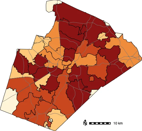
See also a dedicated tutorial on Making Thematic Maps.
Summary
Using the North Carolina schools, roads, and ZIP codes, we have worked through the core vector toolkit in GRASS:
- exploring features and attributes with
v.infoandv.db.select, - selecting by attribute (
v.extract) and by location (v.select), - buffering (
v.buffer) and overlaying (v.overlay) layers, and - counting points per area (
v.vect.stats) for a thematic map.