# Get general average and SD
methods=["average", "stddev"]

for me in methods:
    gs.run_command("t.rast.series",
                   input="lst_daily",
                   method=me,
                   output=f"lst_{me}",
nprocs=6)Temporal algebra
time series
raster
advanced
Python
Demonstrate the use of GRASS temporal algebra tools to estimate anomalies and phenology related variables.
In this third part of the time series tutorials, we will go through different temporal algebra examples. There are five modules within the temporal framework that allow us to perform temporal map algebra on different types of data: t.rast.mapcalc, t.rast.algebra, t.rast3d.mapcalc, t.rast3d.algebra, and t.vect.algebra. We will focus on the raster oriented tools in this tutorial.
NoteSetup
This tutorial can be run locally or in Google Colab. However, make sure you install GRASS 8.4+, download the LST sample data and set up your project as explained in the first time series tutorial.
What tool to use?
Both t.rast.mapcalc and t.rast.algebra allow us to perform spatio-temporal operations on temporally sampled maps of raster time series (STRDS). Also, both tools support spatial and temporal functions.
Spatial operators and functions are those used in r.mapcalc.
Temporal internal variables supported for both relative and absolute time include: td() (time delta), start_time() and end_time(). There are also several useful internal temporal variables supported especially for absolute time, e.g.: start_doy(), start_year(), start_month() and so on.
Both t.rast.mapcalc and t.rast.algebra support temporal operations. However, only t.rast.algebra is effectively temporally aware; t.rast.mapcalc is mostly a wrapper around r.mapcalc. Indeed, t.rast.algebra is able to perform a wide range of temporal operations based on the temporal topology of maps within STRDS. Supported operators, relations and functions are shown in the table below.
| Category | Examples |
|---|---|
| Temporal operators | u (union), i (intersection), l (left reference), etc. |
| Temporal relations | equals, during, contains, starts, etc. |
| Temporal selection | :, !: |
| Temporal functions | td(), start_time(), start_doy(), #, tmap(), map(), t_snap(), buff_t(), t_shift(), etc. |
| Temporal neighborhood modifier | [x,y,t] |
| Spatial operators | +, -, *, /, % |
| Spatial functions | abs(x), float(x), int(x), log(x), round(x), isnull(x), null(), etc. |
They can all be combined in nested expressions with conditions statements to create spatio-temporal operators! In general, expressions have the following structure: {"spatial or select operator", "temporal relations", "temporal operator"} and they can be combined with conditional statements such as: if(topologies, conditions, A, B) where A and B can be either space time datasets or expressions (e.g., A+B). Just for illustration purposes, let’s see some examples from the manual page.
| Expression | Description |
|---|---|
C = A {+,equal,l} B |
C will have the same time stamps as A and will be A + B for maps with equal time stamps. Equivalent to C = A + B. The default temporal relation is equal and the default temporal operator is left reference. |
C = if(start_date(A) < "2005-01-01", A + B) |
C will be A + B if the start date of A is earlier than January 1, 2005. This is an if-then conditional expression. |
C = if({equal}, A > 100 && A < 1600 {&&,equal} td(A) > 30, B) |
C will include all cells from B with equal temporal relations to A, if values of A are between 100 and 1600 in time intervals longer than 30 units. Equivalent to C = if(A > 100 && A < 1600 && td(A) > 30, B). |
C = A {:, during} tmap(event) |
C will include all maps from A that occur during the temporal extent of the single map event. |
C = A * map(constant_value) |
C will include all raster maps from A multiplied by a raster map called constant_value (a map without a time stamp). |
B = if(A > 0.0 && A[-1] > 0.0 && A[-2] > 0.0, start_doy(A, 0), 0) |
B will contain the Day of Year (DOY) from A where three consecutive time intervals have values > 0. Otherwise, B will contain 0. |
Let’s see some examples using the LST daily time series from northern Italy. We start with something simple to refresh what we learnt in the tutorial about aggregations.
Anomalies
To estimate annual anomalies, we need the long term average (\(Avg\)) and standard deviation (\(SD\)) of the whole series, and the annual averages (\(Avg_i\)). Then, we estimate the standardized anomalies as:
\[ StdAnom_i = \frac{Avg_i - Avg}{SD} \]
Let’s first obtain the average and standard deviation for the series:
and then the annual LST average:
# Get annual averages
gs.run_command("t.rast.aggregate",
               input="lst_daily",
               method="average",
               granularity="1 years",
               output="lst_annual_average",
               basename="lst_average",
               suffix="gran",
               nprocs=6)
We now use t.rast.algebra to estimate the anomalies.
# Estimate annual anomalies
expression="lst_annual_anomaly = (lst_annual_average - map(lst_average)) / map(lst_stddev)"

gs.run_command("t.rast.algebra",
               expression=expression,
               basename="lst_annual_anomaly",
               suffix="gran",
               nprocs=6) # change accordingly!
We set the differences color palette for the whole time series and then create an animation.
# Set difference color table
gs.run_command("t.rast.colors",
               input="lst_annual_anomaly",
               color="difference")
# Animation of annual anomalies
anomalies = gj.TimeSeriesMap()
anomalies.add_raster_series("lst_annual_anomaly", fill_gaps=False)
anomalies.d_legend(color="black", at=(5, 50, 2, 6))
anomalies.show()# Save animation
anomalies.save("anomalies.gif")
Month with maximum LST
We will use t.rast.mapcalc to obtain the month when the maximum LST occurred during our study period. We already estimated the map with the maximum LST in the temporal aggregations tutorial, but let’s refresh our memories:
gs.run_command("t.rast.series",
               input="lst_daily",
               output=f"lst_maximum",
               method="maximum",
               nprocs=4)
Then, we use t.rast.mapcalc to compare all maps in lst_daily time series with the lst_maximum map and save the month only when there’s a match. The result will probably be a very sparse time series.
# Get time series with month of maximum LST
expression="if(lst_daily == lst_maximum, start_month(), null())"

gs.run_command("t.rast.mapcalc",
               flags="n", # register also null maps
               inputs="lst_daily",
               output="month_max_lst",
               basename="month_max_lst",
               expression=expression,
               nprocs=6) # change accordingly!
# Get basic info
print(gs.read_command("t.info", input="month_max_lst"))Now we can aggregate our sparse time series to obtain the earliest month in which the maximum LST occurred.
# Get the earliest month in which the maximum appeared (method=minimum)
gs.run_command("t.rast.series",
               input="month_max_lst",
               method="minimum",
               output="max_lst_date",
               nprocs=6)
We remove the intermediate time series as we were only interested in the resulting aggregated map. For that we use the tool t.remove that allow us to control what to remove depending on the combination of flags we use. In this case, we want to remove both the time series and maps within it, so we use d to remove the STRDS, unregister maps from temporal database and delete them from mapset, and f to actually force the removal.
# Remove month_max_lst strds
gs.run_command("t.remove",
               flags="df",
               inputs="month_max_lst")

# Check it's gone
print(gs.read_command("t.list"))
Let’s display the result using the Map class from grass.jupyter package:
mm = gj.Map()
mm.d_rast(map="max_lst_date")
mm.d_vect(map="italy_borders_0", type="boundary", color="#4D4D4D", width=2)
mm.d_legend(raster="max_lst_date", title="Month", fontsize=12, at=(2, 35, 1, 20), border_color="white", flags="b")
mm.d_barscale(length=50, units="kilometers", segment=4, fontsize=14, at=(80, 8))
mm.d_northarrow(at=(95, 19))
mm.d_text(text="Month of maximum LST", color="black", font="sans", size=4, bgcolor="white")
mm.show()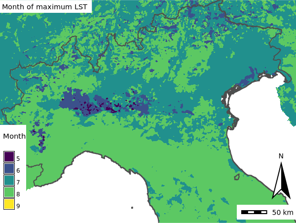
Number of days with LST >= 20 and <= 30
Some plague insects tend to thrive in a certain range of temperatures. Let’s assume this range is from 20 to 30 °C. Here, we’ll estimate the number of days within this range per year, and then, we’ll estimate the median along years.
# Keep only pixels meeting the condition
expression="lst_higher20_lower30 = if(lst_daily >= 20.0 && lst_daily <= 30.0, 1, null())"

gs.run_command("t.rast.algebra",
               expression=expression,
               basename="lst_higher20_lower30",
               suffix="gran",
               nproc=6,
               flags="n")
# Count how many times per year the condition is met
gs.run_command("t.rast.aggregate",
input="lst_higher20_lower30",
output="count_lst_higher20_lower30",
basename="count_lst_higher20_lower30",
suffix="gran",
method="count",
granularity="1 years")# Check raster maps in the STRDS
gs.run_command("t.rast.list",
input="count_lst_higher20_lower30",
columns="name,start_time,min,max")# Median number of days with average lst >= 20 and <= 30
gs.run_command("t.rast.series",
input="count_lst_higher20_lower30",
output="median_count_lst_higher20_lower30",
method="median")# Display raster map with interactive class
h20_map = gj.InteractiveMap()
h20_map.add_raster("median_count_lst_higher20_lower30")
h20_map.show()
CautionQuestion
How would you check if the median number of days with lst >= 20 and <= 30 is changing along the years?
Number of consecutive days with LST <= -10.0
Likewise, there are temperature thresholds that mark a limit to insects survival. Here, we’ll use the lowest temperature threshold. Most importantly, we we’ll count the number of consecutive days with temperatures below this threshold.
We’ll use again the temporal algebra and we’ll recall the concept of topology that we defined at the beginning of these tutorials. First, we need to create a STRDS of annual granularity that will contain only zeroes. This annual STRDS, that we call annual_mask, will be our base to add the value 1 each time the condition < -10 °C in consecutive days is met. Finally, we estimate the median number of days with LST lower than -10 °C over the 5 years.
# Create annual mask
gs.run_command("t.rast.aggregate",
               input="lst_daily",
               output="annual_mask",
               basename="annual_mask",
               suffix="gran",
               granularity="1 year",
               method="count")
# Replace values by zero
expression="if(annual_mask, 0)"
gs.run_command("t.rast.mapcalc",
input="annual_mask",
output="annual_mask_0",
expression=expression,
basename="annual_mask_0")# Calculate consecutive days with LST <= -10.0
expression="lower_m10_consec_days = annual_mask_0 {+,contains,l} if(lst_daily <= -10.0 && lst_daily[-1] <= -10.0 || lst_daily[1] <= -10.0 && lst_daily <= -10.0, 1, 0)"
gs.run_command("t.rast.algebra",
expression=expression,
basename="lower_m10",
suffix="gran",
nproc=6)# Inspect values
gs.run_command("t.rast.list",
input="lower_m10_consec_days",
columns="name,start_time,min,max")# Median number of consecutive days with LST <= -10
gs.run_command("t.rast.series",
input="lower_m10_consec_days",
output="median_lower_m10_consec_days",
method="median")# Display raster map with interactive class
lt10_map = gj.InteractiveMap()
lt10_map.add_raster("median_lower_m10_consec_days")
lt10_map.show()References
- Gebbert, S., Pebesma, E. 2014. TGRASS: A temporal GIS for field based environmental modeling. Environmental Modelling & Software 53, 1-12. DOI.
- Gebbert, S., Pebesma, E. 2017. The GRASS GIS temporal framework. International Journal of Geographical Information Science 31, 1273-1292. DOI.
- Gebbert, S., Leppelt, T., Pebesma, E., 2019. A topology based spatio-temporal map algebra for big data analysis. Data 4, 86. DOI.
- Temporal data processing wiki page.
The development of this tutorial was funded by the US National Science Foundation (NSF), award 2303651.