# Daily to monthly
gs.run_command("t.rast.aggregate",
                input="lst_daily",
                method="average",
                granularity="1 months",
                basename="lst_avg",
                output="lst_monthly",
                suffix="gran",
nprocs=4)Time series aggregation
time series
raster
advanced
Python
Tutorial on different types of raster time series aggregations, i.e., with granularity, full series, long term averages, and their visualization.
In this second time series tutorial, we will go through different ways of performing aggregations. Temporal aggregation is a very common task when working with time series as it allows us to summarize information and find patterns of change both in space and time.
NoteSetup
This tutorial can be run locally or in Google Colab. However, make sure you install GRASS 8.4+, download the sample data and set up your project as explained in the first time series tutorial.
There are two main tools to do time series aggregations in GRASS: t.rast.aggregate and t.rast.series. We’ll demonstrate their usage in the upcoming sections.
Aggregation with granularity
Granularity is the greatest common divisor of the temporal extents (and possible gaps) of all maps in a space-time dataset. To perform time series aggregation with granularity, we use t.rast.aggregate. This tool allows us to aggregate our time series into larger granularities, i.e., from hourly to daily, from daily to weekly, monthly, etc. It also permits to aggregate with ad hoc granularities like 3 minutes, 5 days, 3 months, etc. Supported aggregate methods include average, minimum, maximum, median, etc. See the r.series manual page for more details.
If you are working with data representing absolute time, t.rast.aggregate will shift the start date for each aggregation process depending on the provided temporal granularity as follows:
- years: will start at the first of January, hence 14-08-2012 00:01:30 will be shifted to 01-01-2012 00:00:00
- months: will start at the first day of a month, hence 14-08-2012 will be shifted to 01-08-2012 00:00:00
- weeks: will start at the first day of a week (Monday), hence 14-08-2012 01:30:30 will be shifted to 13-08-2012 01:00:00
- days: will start at the first hour of a day, hence 14-08-2012 00:01:30 will be shifted to 14-08-2012 00:00:00
- hours: will start at the first minute of a hour, hence 14-08-2012 01:30:30 will be shifted to 14-08-2012 01:00:00
- minutes: will start at the first second of a minute, hence 14-08-2012 01:30:30 will be shifted to 14-08-2012 01:30:00
The specification of the temporal relation between the aggregation intervals and the raster map layers to be aggregated is always formulated from the aggregation interval viewpoint. By default, it is set to the contains relation to aggregate all maps that are temporally within an aggregation interval.
NoteTemporal topology
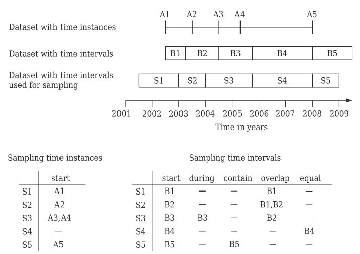
Temporal topology refers to the temporal relations among time intervals or instances in different time series. They are mostly useful when sampling one STRDS with another (see t.sample manual). Some examples of temporal relations are start, equal, during, contain, overlap, etc. See below a graphic representation of relations and sampling taken from Gebbert and Pebesma (2014). Note that A1 starts in S1, B3 is during S3, B4 equals S4, B1 overlaps S1.
Monthly and seasonal averages
To demonstrate the basic usage of t.rast.aggregate, let’s create monthly and seasonal time series starting from the lst_daily time series we created in the time series management tutorial.
# Daily to (sort of) seasonal
gs.run_command("t.rast.aggregate",
                input="lst_daily",
                method="average",
                granularity="3 months",
                basename="lst_avg",
                output="lst_seasonal",
                suffix="gran",
                nprocs=4)
If we would like to follow the so called meteorological seasons, i.e., that spring started with March, then we could have used the where option to shift the starting point of the aggregation period as follows: where="start_time >= '2013-03-01 00:00:00'".
Let’s compare the granularities using the timeline plot…
!g.gui.timeline lst_monthly,lst_seasonal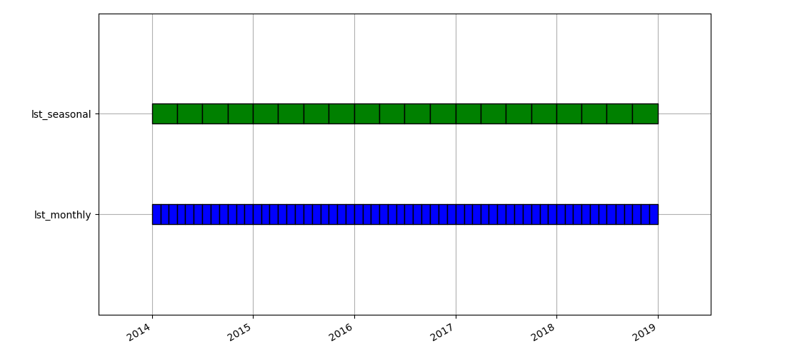
and use grass.jupyter to create a nice animation of the seasonal time series:
lstseries = gj.TimeSeriesMap()
lstseries.add_raster_series("lst_seasonal", fill_gaps=False)
lstseries.d_legend(color="black", at=(5, 50, 2, 6))
lstseries.show()
# Optionally, write out to animated GIF
lstseries.save("lstseries.gif")For astronomical seasons, i.e., those defined by solstices and equinoxes, we can use t.rast.aggregate.ds as in this example, or for an approximate result:
gs.run_command("t.rast.aggregate",
                input="lst_daily",
                method="average",
                where="start_time >= '2013-03-21 00:00:00'",
                granularity="3 months",
                basename="lst_avg",
                output="lst_seasonal",
                suffix="gran",
                nprocs=4)
# Check info
gs.read_command("t.info", input="lst_seasonal")# Check raster maps in the STRDS
gs.run_command("t.rast.list", input="lst_seasonal")Spring warming
We define spring warming as the velocity with which temperature increases from winter into spring and we can approximate it as the linear regression slope among LST values of February, March and April. Let’s see how to use t.rast.aggregate to estimate yearly spring warming values.
# Define list of months
months = [f"{m:02d}" for m in range(2, 5)]
print(months)
# Annual spring warming
gs.run_command("t.rast.aggregate",
input="lst_daily",
output="annual_spring_warming",
basename="spring_warming",
suffix="gran",
method="slope",
granularity="1 years",
where=f"strftime('%m',start_time)='{months[0]}' or strftime('%m',start_time)='{months[1]}' or strftime('%m', start_time)='{months[2]}'")# Check raster maps in the STRDS
gs.run_command("t.rast.list", input="annual_spring_warming")spring_warming = gj.TimeSeriesMap()
spring_warming.add_raster_series("annual_spring_warming", fill_gaps=False)
spring_warming.d_legend(color="black", at=(5, 50, 2, 6))
spring_warming.show()
CautionQuestion
How would you obtain the average spring warming over the whole time series?
# Average spring warming
gs.run_command("t.rast.series",
               input="annual_spring_warming",
               output="avg_spring_warming",
               method="average")

# Display raster map with interactive class
spw_map = gj.InteractiveMap(width = 500, use_region=True, tiles="CartoDB.DarkMatter")
spw_map.add_raster("avg_spring_warming")
spw_map.add_layer_control(position = "bottomright")
spw_map.show()
Full series aggregation
The tool t.rast.series allows us to aggregate complete time series (or only selected parts) with a certain method. Available aggregation methods include average, minimum, maximum, median, etc. See the r.series manual page for details.
Maximum and minimum LST
We’ll demonstrate how to aggregate the whole lst_daily time series to obtain the maximum and minimum LST value for the period 2014-2018. Note that the input is a STRDS object while the output is a single map in which pixel values correspond to the maximum or minimum value of the time series they represent.
# Get maximum and minimum LST in the STRDS
methods = ["maximum", "minimum"]

for m in methods:
    gs.run_command("t.rast.series",
                   input="lst_daily",
                   output=f"lst_{m}",
                   method=m,
                   nprocs=4)
# Change color palette to Celsius
gs.run_command("r.colors",
map="lst_minimum,lst_maximum",
color="celsius")Let’s use the InteractiveMap class from grass.jupyter to visualize the maximum and minimum LST maps.
# Plot
lst_map=gj.InteractiveMap()
lst_map.add_raster("lst_minimum")
lst_map.add_raster("lst_maximum")
lst_map.show()
Long term aggregations
If we want to know the temperature on a “typical” January, February and so on, we estimate the so called long-term averages or climatologies for each month. These are usually computed over 20 or 30 years of data, but for the purpose of demonstrating the usage of t.rast.series for long term aggregations, we will use our 5-year time series here.
We will use what we learned in the listing and selection examples in the first time series tutorial, i.e., we need to select all maps for each month to perform the aggregation. So, the input will be the whole time series, but we will use only some maps to estimate the long term monthly average, minimum and maximum values. Let’s see how to do all that with a simple for loop over months and methods:
# Estimate long term aggr for all months and methods
months = [f"{m:02d}" for m in range(1, 13)]
methods = ["average", "minimum", "maximum"]

for month in months:
    print(f"Aggregating all {month} maps")
    gs.run_command("t.rast.series",
                   input="lst_daily",
                   method=methods,
                   where=f"strftime('%m', start_time)='{month}'",
                   output=[f"lst_{method}_{month}" for method in methods])
# List newly created maps
map_list = gs.list_grouped(type="raster", pattern="*{average,minimum,maximum}*")['italy_LST_daily']Let’s create an animation of the long term average LST.
# List of average maps
map_list = gs.list_grouped(type="raster", pattern="*_average_*")['italy_LST_daily']

# Animation with SeriesMap class
series = gj.SeriesMap()
series.add_rasters(map_list)
series.d_barscale()
series.show()
CautionQuestion
Why didn’t we list with t.rast.list?
Bioclimatic variables
Perhaps you have heard of Worldclim or CHELSA bioclimatic variables? Well, these are 19 variables that represent potentially limiting conditions for species. They derive from the combination of temperature and precipitation long term aggregations. Let’s use those that we estimated in the previous example to estimate the bioclimatic variables that include temperature. GRASS has a nice extension, r.bioclim, to estimate bioclimatic variables.
# Install extension
gs.run_command("g.extension", extension="r.bioclim")
# Get lists of maps needed
tmin = gs.list_grouped(type="raster", pattern="lst_minimum_??")["italy_LST_daily"]
tmax = gs.list_grouped(type="raster", pattern="lst_maximum_??")["italy_LST_daily"]
tavg = gs.list_grouped(type="raster", pattern="lst_average_??")["italy_LST_daily"]
print(tmin, tmax, tavg)# Estimate temperature related bioclimatic variables
gs.run_command("r.bioclim",
tmin=tmin,
tmax=tmax,
tavg=tavg,
output="worldclim_")# List output maps
gs.list_grouped(type="raster", pattern="worldclim*")["italy_LST_daily"]Let’s have a look at some of the maps we just created:
# Display raster map with interactive class
bio_map = gj.InteractiveMap()
bio_map.add_raster("worldclim_bio01")
bio_map.add_raster("worldclim_bio02")
bio_map.show()
Let’s assume a certain insect species can only survive where winter mean temperatures are above 5 degrees. How would you determine suitable areas? We’ll see that in the upcoming tutorial, stay tuned!
Tip
If you are curious, maybe you want to have a look at t.rast.mapcalc and t.rast.algebra and try to come up with a solution.
References
- Gebbert, S., Pebesma, E. 2014. TGRASS: A temporal GIS for field based environmental modeling. Environmental Modelling & Software 53, 1-12. DOI.
- Gebbert, S., Pebesma, E. 2017. The GRASS GIS temporal framework. International Journal of Geographical Information Science 31, 1273-1292. DOI.
- Temporal data processing wiki page.
The development of this tutorial was funded by the US National Science Foundation (NSF), award 2303651.