r.colors -e map=elevation color=elevationVisualizing and Modeling Terrain from DEMs in GRASS
beginner
intermediate
raster
DEM
visualization
terrain
slope
aspect
landforms
hydrology
streams
This tutorial guides a user through multiple ways of analyzing and modeling terrain from DEM raster maps.
GRASS has many tools that can help you visualize and model terrain from digital elevation model (DEM) raster maps. A few examples include:
r.shade for visualization,
r.slope.aspect for modeling slope and aspect,
r.geomorphon for modeling topographic features,
r.watershed for modeling overland flow and watershed basins, and
r.stream.extract to generate stream networks.
This tutorial will explore these tools, but they are only a few of the many GRASS modules to represent and analyze landscapes.
NoteDemo Dataset
This tutorial uses one of the standard GRASS sample data sets for Flagstaff, Arizona, USA: flagstaff_arizona_usa. We will refer to place names in that data set, but it can be completed with any of the standard sample data sets for any region–for example, the North Carolina data set. We will use the elevation DEM.
NoteGRASS interfaces
This tutorial is designed so that you can complete it using the GRASS GUI, GRASS commands from the console or terminal, or using GRASS commands in a Jupyter Notebook environment.
NoteDon’t know how to get started?
If you are not sure how to get started with GRASS using its graphical user interface or using Python, checkout the tutorials Get started with GRASS GUI and Get started with GRASS & Python in Jupyter Notebooks.
Terrain, DEMs, and Raster GIS
- While many maps represent features with vector points, lines, and areas, the spatially continuous landscape of terrain is often represented in GIS by rasters.

- Rasters represent terrain by a continuous grid of cells, much like the pixels in a digital photo.
- With a digital elevation model (DEM) raster, each grid cell stores the elevation above sea level of the terrain covered by the grid cell.
By storing the elevation of a terrain at multiple points, a DEM can be used to calculate slope and aspect at every location, to identify topographic features, or to model which way water will flow over a terrain.
It can also be used to produce striking visualizations that display terrain characteristics, as well as representing topography.
In this tutorial, we will use the DEM named elevation. In the Flagstaff sample data set, this DEM has a spatial resolution of 30m (grid cells represent 30x30m patches of the terrain) with elevation in meters above mean sea level.
Visualizing Terrain
There are several ways to create terrain visualizations in GRASS.
A color table can be applied to a DEM so that different elevations are assigned to different colors.
A DEM can be shaded to create the appearance of 3D topographic relief.
Color can be applied to a shaded relief map.
A DEM of terrain can be rendered in 3D to be visualized from different perspectives.
Applying a color table to a DEM
GRASS offers multiple ways to apply color to a DEM to visualize terrain under the Raster/Manage colors menu. The simplest way is to apply a color table using the r.colors module.
Let’s apply the elevation color table to the Flagstaff DEM. This color table assigns ‘hot’ colors to higher elevations and ‘cool’ colors to lower elevations.
Select r.colors tool from the Raster/Manage colors menu.
In the “Map” tab, select elevation map in the “Name of raster map(s)” entry box.

In the Define tab, select elevation as the color table.
Click Run.

Try out some other color tables. ETOPO2, terrain, and the SRTM color tables are also good for terrain colors. You can also make a custom color table easily, described in the r.colors manual.
gs.run_command("r.colors",
map="elevation",
color="elevation",
flags="e")
Shaded relief of terrain
A shaded relief map adds shadows to a DEM, for a user-specified direction of sunlight and position of the sun above the horizon. Relief shading can be generated because with the terrain elevation stored in each grid cell, the height and aspect (direction the terrain is facing) of each cell is known. A relief map has the appearance of 3D topography.
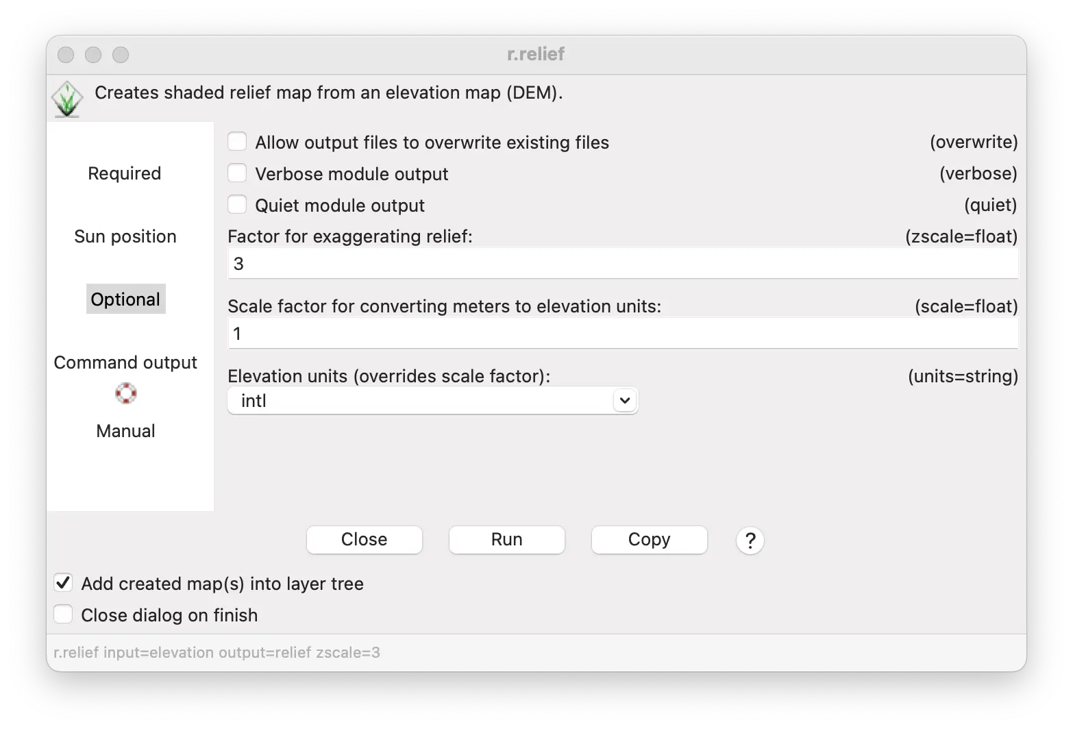
We can use the r.relief tool to visualize the topographic relief of the elevation DEM for the Flagstaff area.
We will keep the defaults for sun direction and height, but increase the vertical exaggeration to 3 to make the topography stand out better.
Raster/Terrain analysis/Compute shaded relief
Select the r.relief tool from the Raster/Terrain analysis/Compute shaded relief menu.
Enter the elevation DEM as the input map.
Enter relief as name for the output.
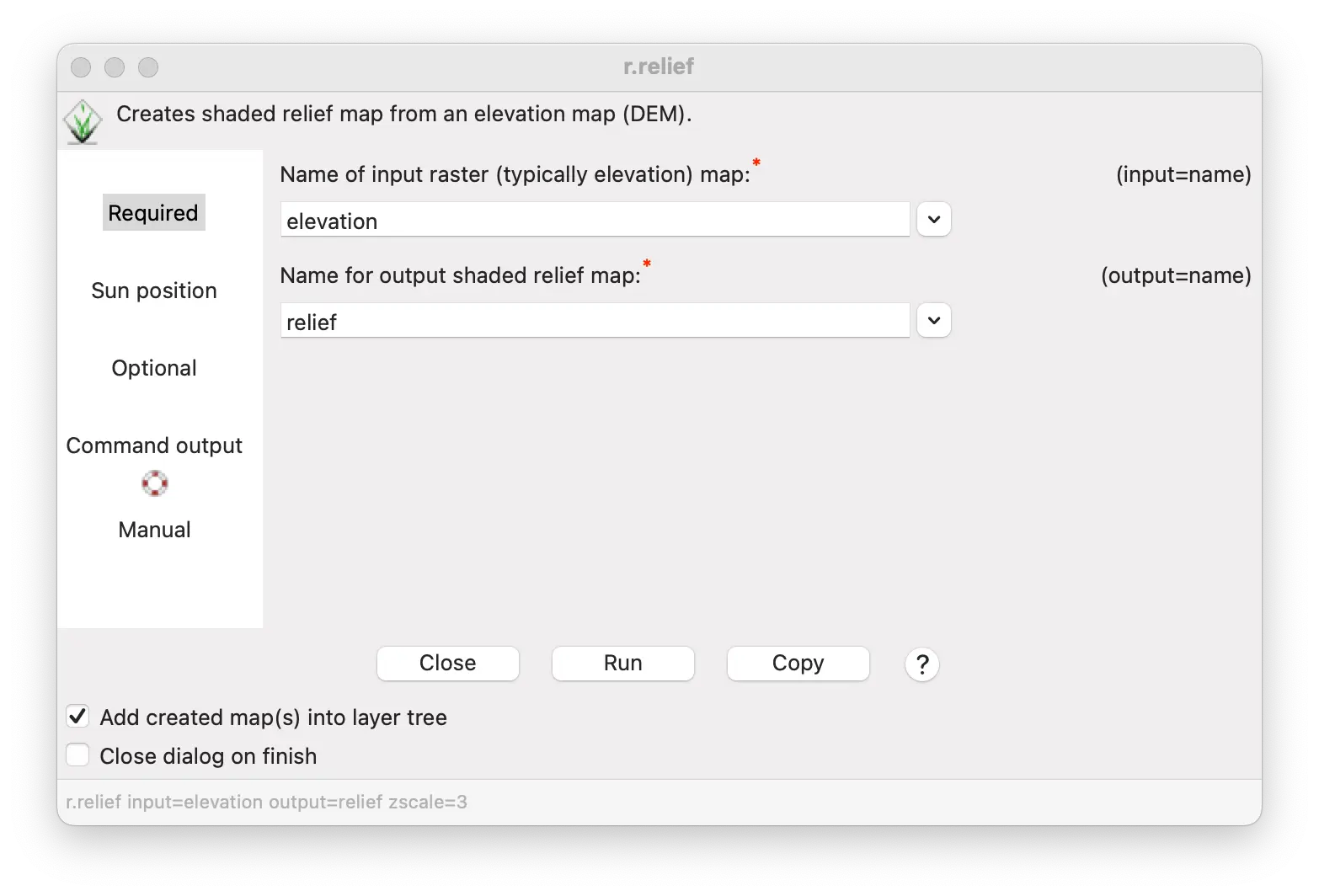
Under the “Optional” tab, enter 3 for the “Factor for exaggerating relief”.
Click Run.
r.relief input=elevation output=relief zscale=3 gs.run_command("r.relief",input="elevation", output="relief" zscale=3)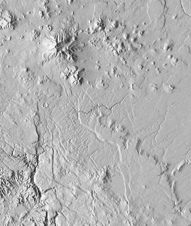
Combining color and relief
To better visualize the difference in the terrain, you can drape the color elevation over the relief map you just made.
GRASS makes it easy for you to fuse color and relief shading to visualize topography, terrain features, land cover, or other geographic information.
This can be done by creating a new map, using r.shade tool or
by dynamically overlaying a color map over a relief map in the GUI layer manager and display window.
We will overlay DEM with the assigned color table from the beginning of this section with the relief map you just made using both methods.
This approach can also be used to visualize other terrain analyses completed later in this tutorial.
We will start by creating a new color-shaded relief map using r.shade.
Open r.shade from the Raster/Terrain analysis/Apply shade to raster menu.
Set “Name of shaded relief” map to to relief.
Set “Name of raster to drape over relief raster” to elevation.
Enter topography_colored_relief as “Name of shaded raster” map.
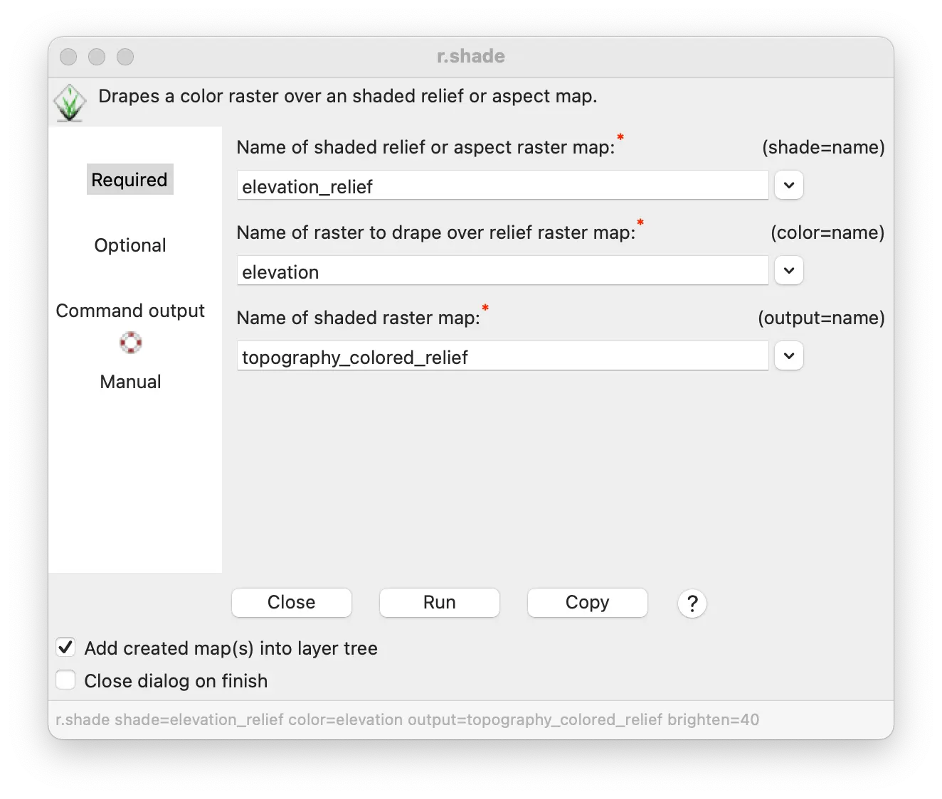
Under the “Optional” tab, set Brightness to 40% to provide a more colorful result.
Click Run.
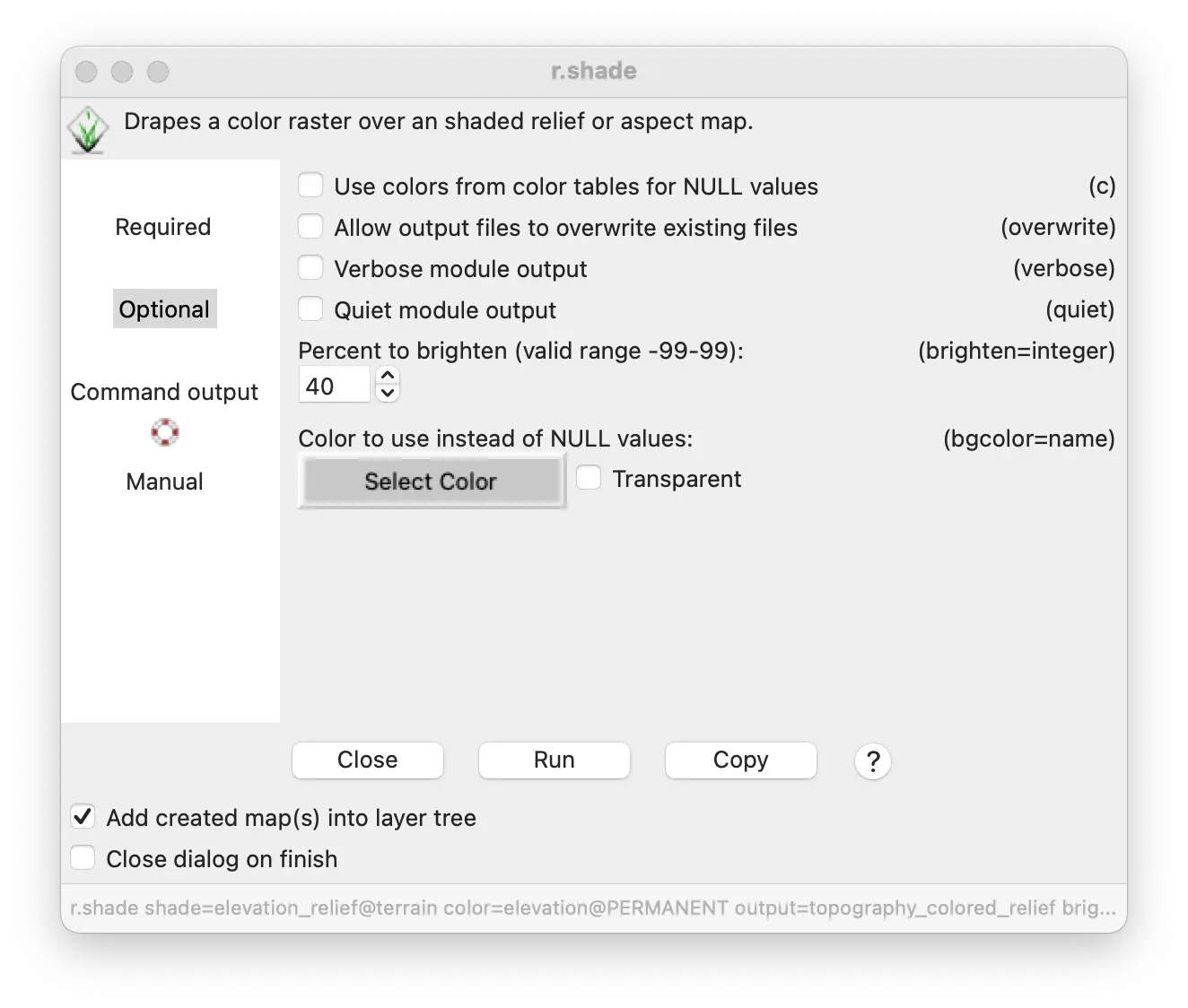
r.shade shade=relief color=elevation output=topography_colored_relief brighten=40gs.run_command("r.shade",
shade="relief,
color="elevation",
output="topography_colored_relief",
brighten=40)
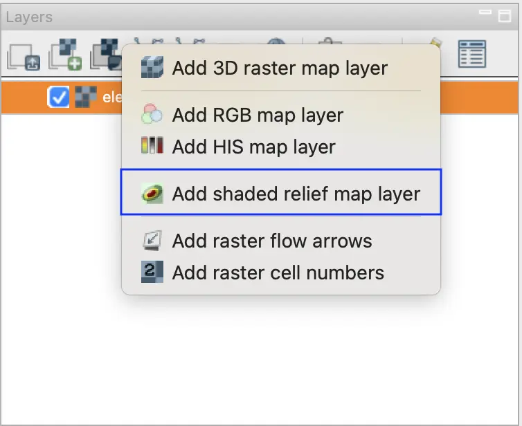
You can also display a color shaded relief map dynamically in the GUI layer manager using the d.shade tool.
In the layer manager, select Add shaded relief map layer (d.shade tool) from the Add various raster map layers menu button.
Enter the relief map into the “Name of shaded relief” text box.
Enter elevation map into the “Name of raster to drape over relief” text box.
If you set the “Percent to brighten” to 30 or 40, it will create a more visually appealing display.
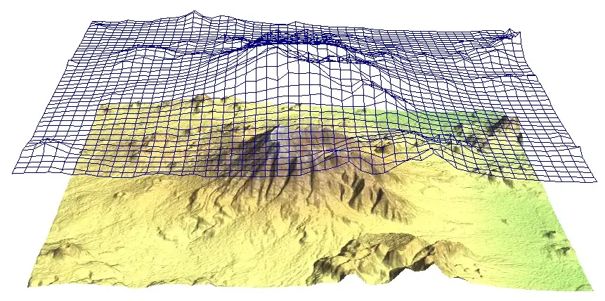
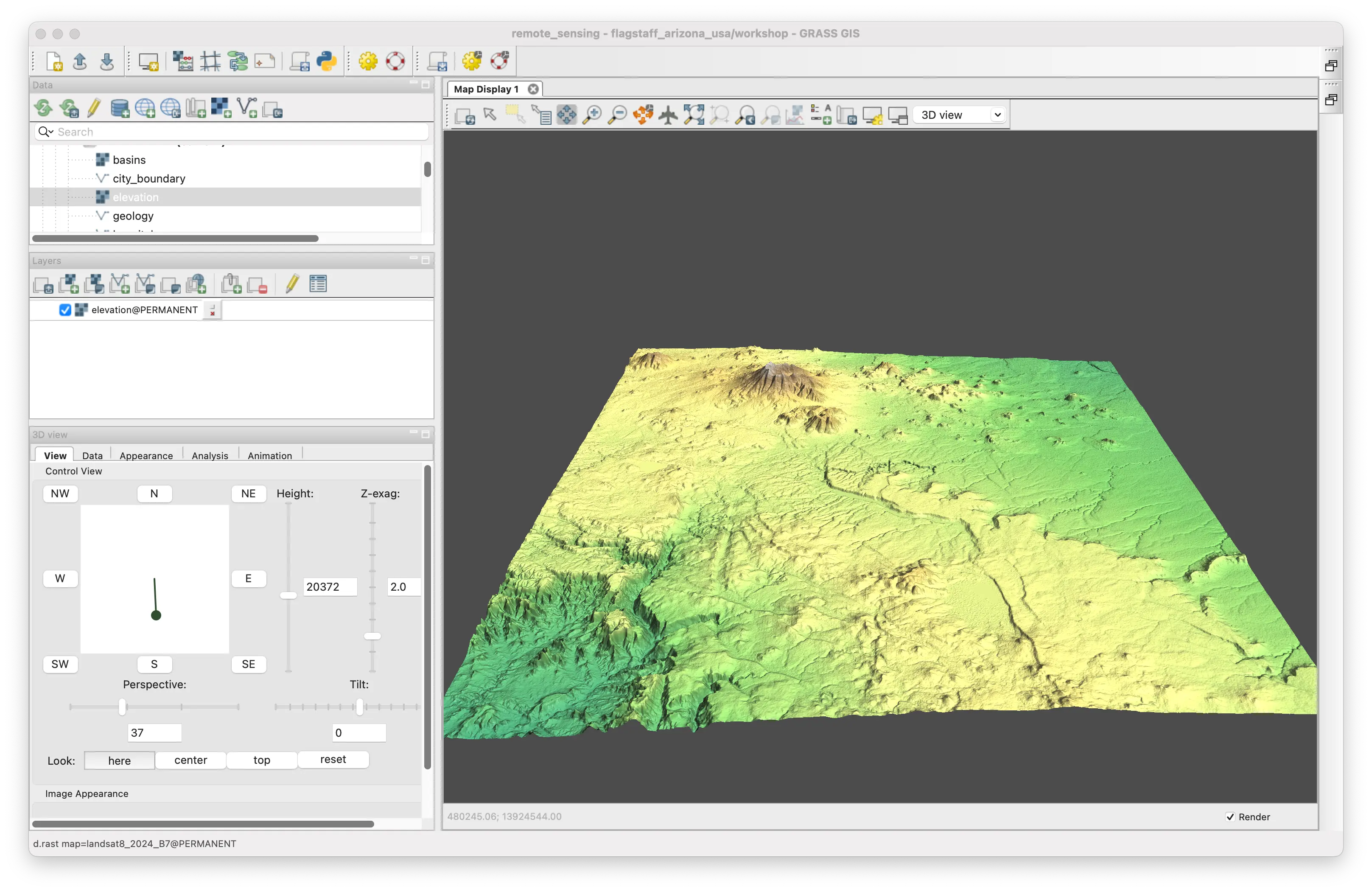
Rendering terrain in 3D
Additionally, a 3D visualization of topography can be rendered in GRASS’s 3D view using the NVIZ module.
Start by opening the elevation DEM in the layer manager. Make sure that no other maps except elevation are displayed.
Select 3D view from the pull-down menu at the top of the map display window.
This should display the elevation map in 3D with the same shading seen in the 2D display.
Use the controls under the “View” tab to change the perspective, z-exaggeration, and other characteristics.
For a more detailed view of the terrain, decrease the “fine” resolution under the “Data” tab.
Analyzing and Modeling Terrain Characteristics
GRASS makes it easy to model and analyze a wide range of terrain characteristics using a DEM. The slope and aspect of terrain, and topographic features like peaks, ridges, and valleys are important for studying and modeling soil features, vegetation, micro-climates, water flow, and movement across the surface. Modeling the way water flows over terrain likewise is relevant for ecology, stream networks, and flood risks. In this tutorial, we will demonstrate how to use a DEM to carry out these analyses.
Slope and aspect
The difference in elevation between a raster cell in a DEM and its surrounding cells, makes it possible to calculate the terrain slope for that cell. It also enables the calculation of the direction that the cell is facing–its aspect.
We can use the same tool r.slope.aspect to determine the slope and aspect, as well as several other terrain characteristics.
We will create new maps from the elevation DEM for slope (each cell will store the slope in degrees) and aspect (each cell will store the aspect in degrees from north).
Open r.slope.aspect tool from the Raster/Terrain analysis/Slope and aspect menu.
Set elevation raster layer as the “Name of input elevation raster map”.
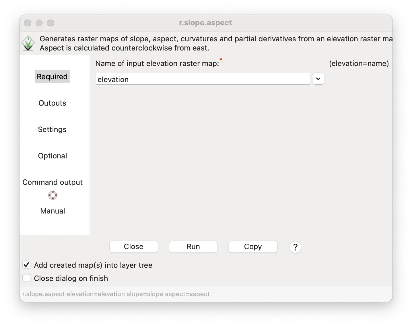
Enter name slope for “Name for output slope raster map”.
Enter name aspect for “Name for output aspect raster map”.
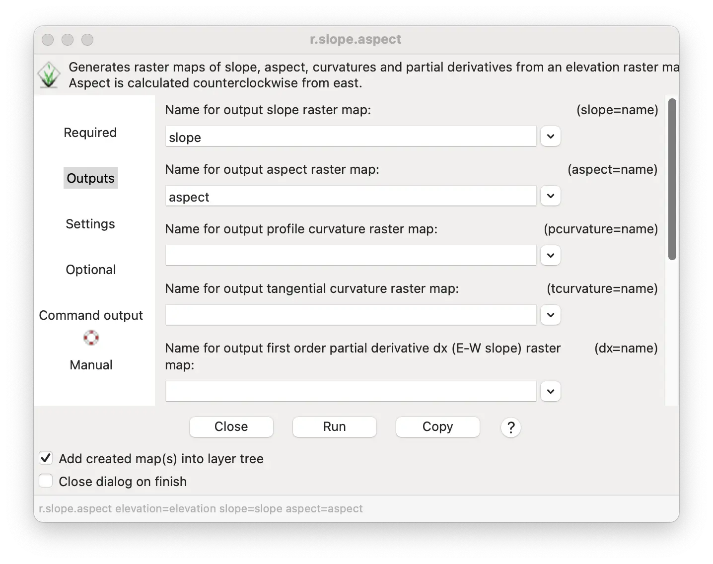
Under the Settings tab, click the checkbox to “Create aspect as degrees clockwise from North”. Otherwise, aspect will be calculated as degrees counter clockwise from East.
Click Run.
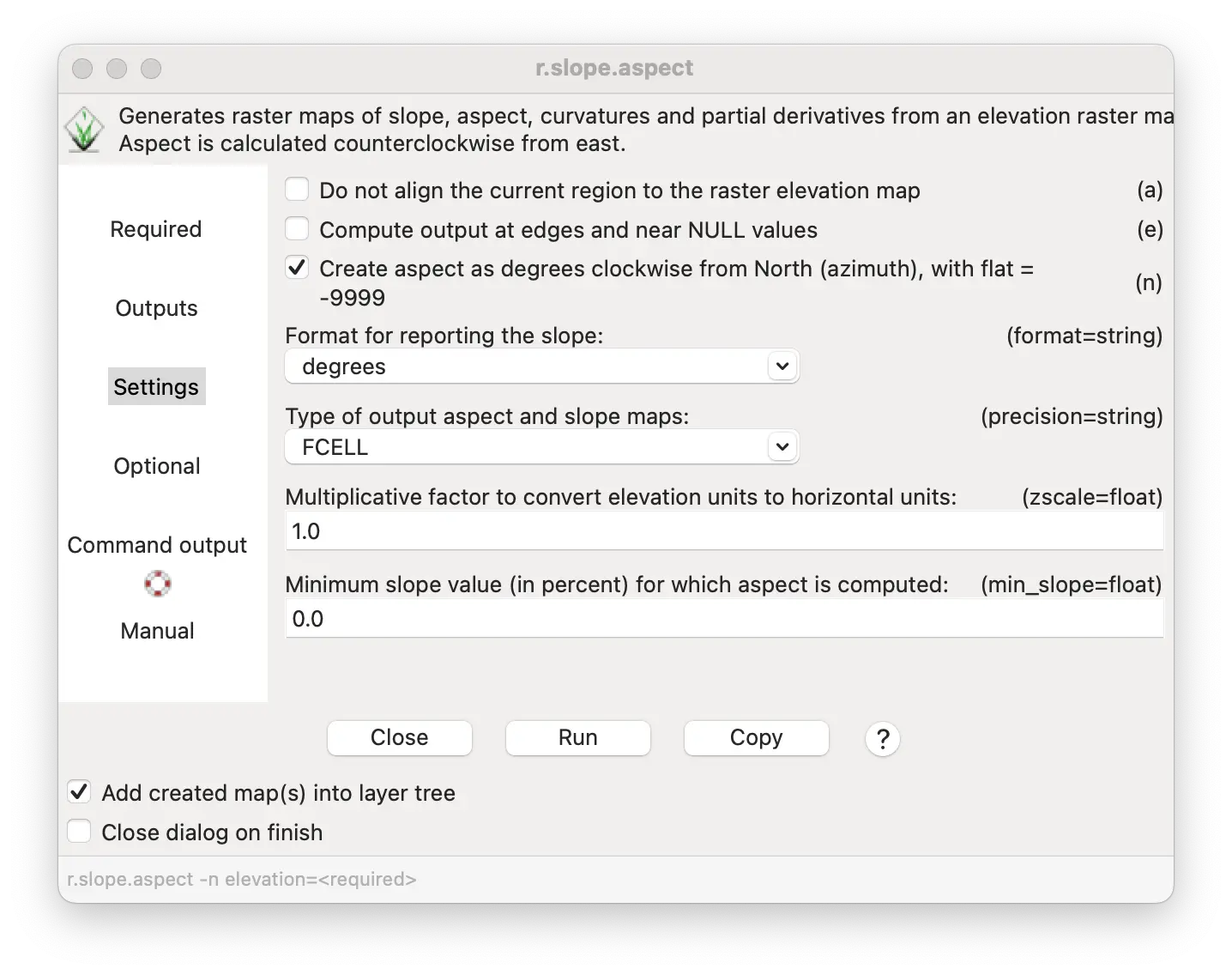
Add the “-n” flag so that aspect will be recorded as degrees clockwise from North. Otherwise, aspect will be calculated as degrees counter clockwise from East.
r.slope.aspect elevation=elevation slope=slope aspect=aspect -nAdd the “-n” flag so that aspect will be recorded as degrees clockwise from North. Otherwise, aspect will be calculated as degrees counter clockwise from East.
gs.run_command("r.slope.aspect",
elevation="elevation",
slope="slope",
aspect="aspect",
flags="n")Here are the resulting slope and aspect maps.
Notice how the default grey scale aspect color table gives the map a 3D appearance, like a relief map. This is because it shades from light to dark according to the orientation of the terrain, much like shadows from the sun. The r.relief tool uses a similar algorithm to generate a relief map.
The r.slope.aspect tool can produce other analytical maps, including maps of the change in slope in the both the downslope and transverse directions, and the rate of change in slope in different directions.
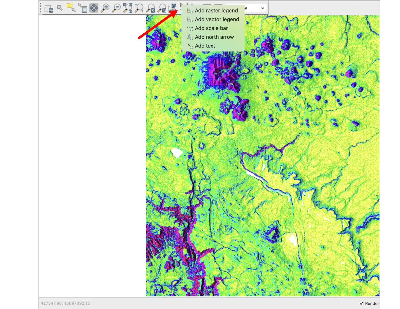
Add a legend to visualization of slope and topography
You can color a relief map with slope using the same procedure described above, but using the slope map for the color rather than the elevation DEM. This will allow you to compare topographic relief and slope.
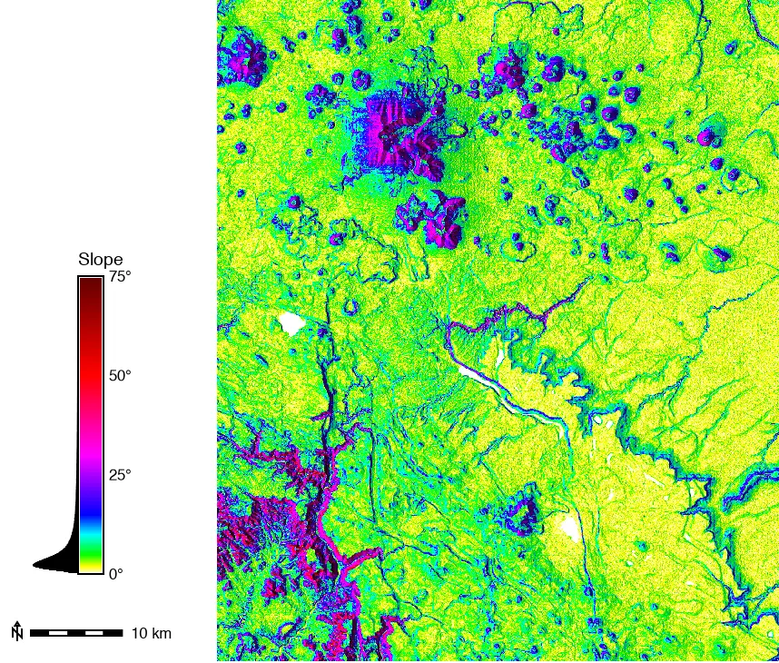
While this may help you visualize the differences between areas, using a legend can help you determine what the range of values present in the raster area and how the colors correspond to these values. With GRASS, you can easily make a highly informative legend for your map.
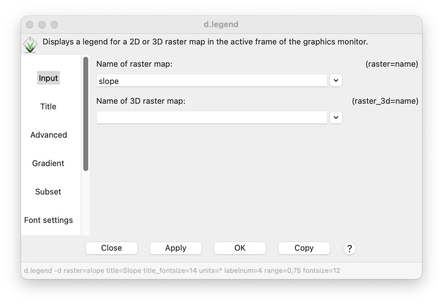
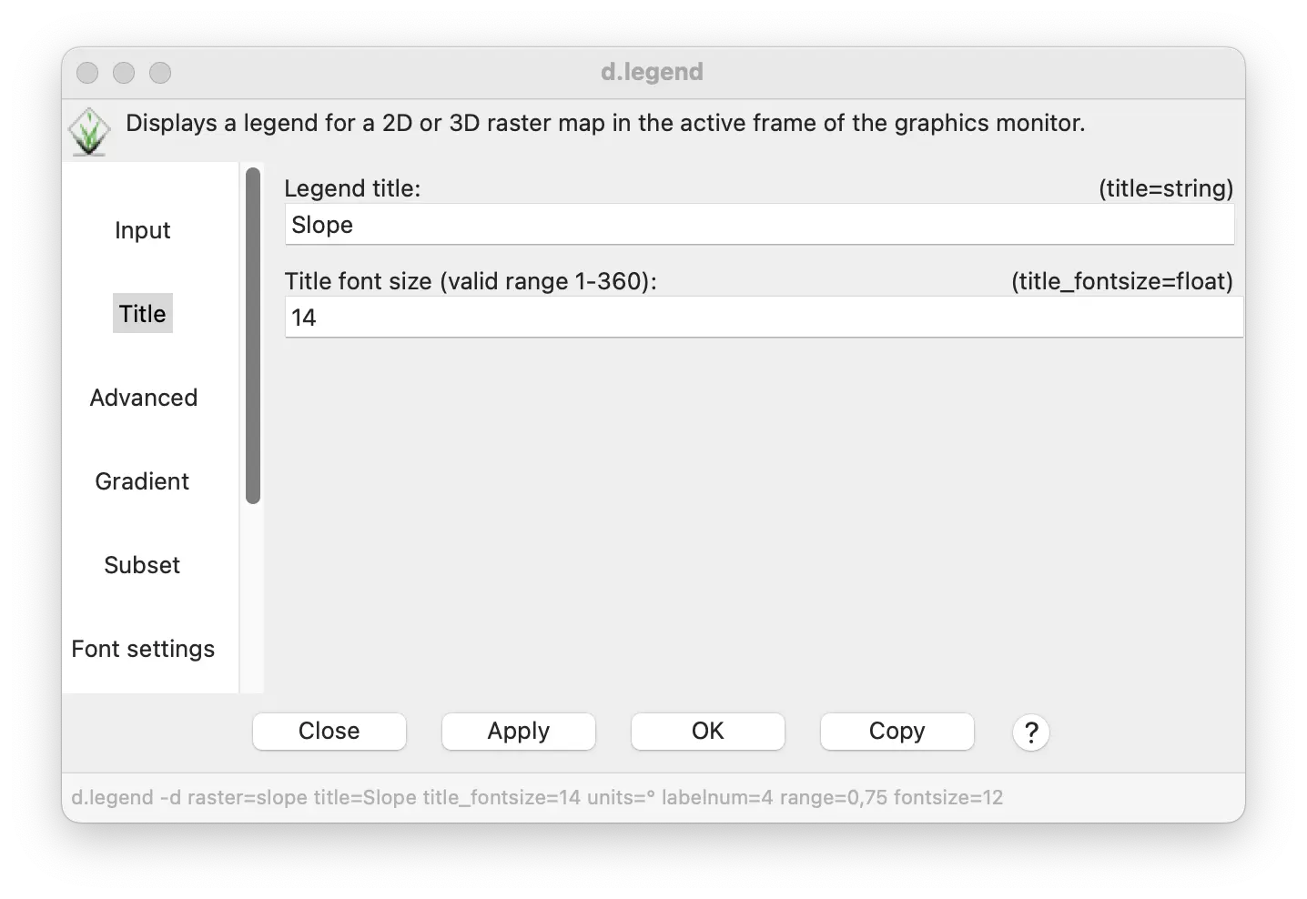
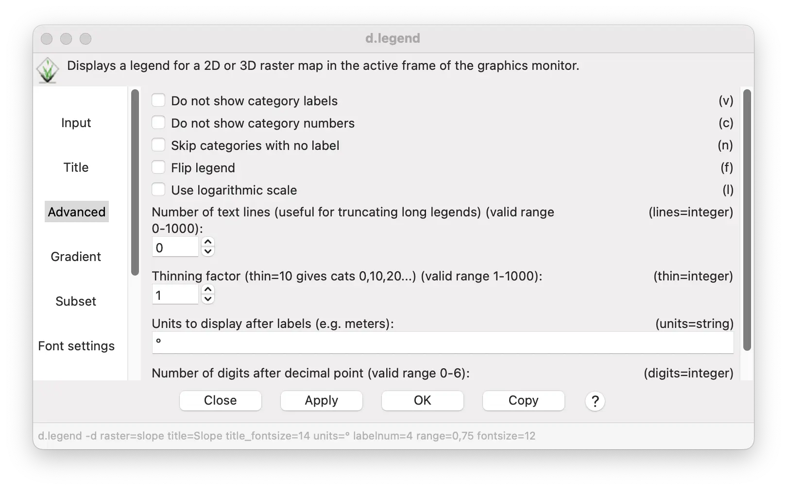
The raster legend tool can be accessed from the display window tool bar. This tool has many options. We’ll explore several of them.
- Under the Input tab, enter slope as the “Name of raster map”.
- Under the Title tab, enter “Slope” as the “Legend title”, and enter 14 as the “Title font size”.
- Under the Advanced tab, enter the degree symbol (°) or the word “deg” as “Units to display”.
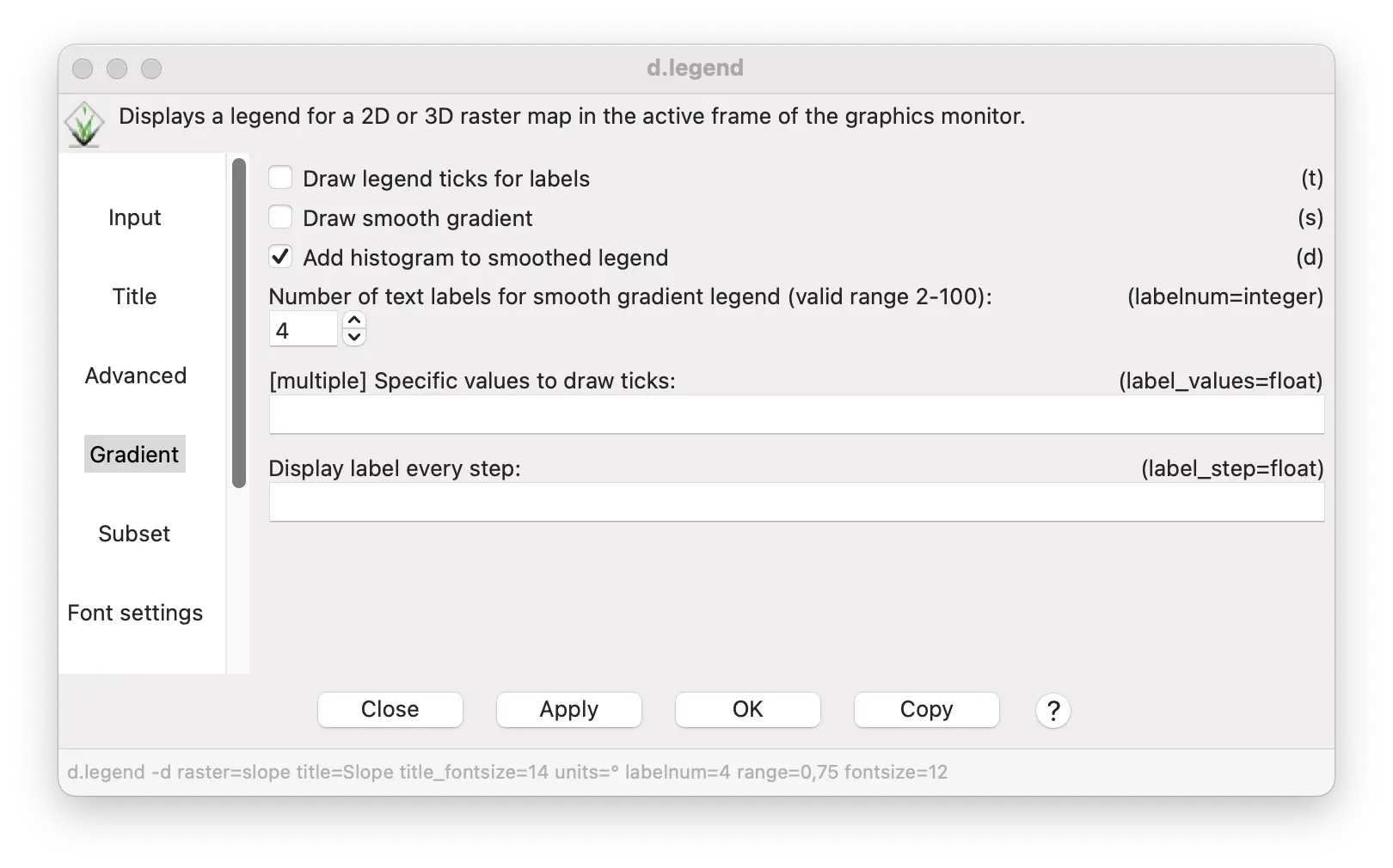
- Under the Gradient tab, check the “Add histogram to smoothed legend” box.
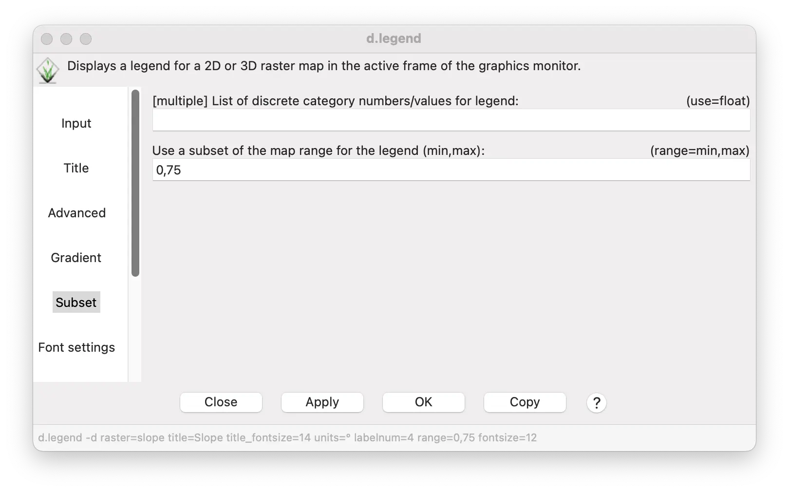
- The maximum slope of the map is 76 degrees. For a nice looking legend, we can limit the display to 0-75 degrees. Under the Subset tab, enter “0,75” in the subset box for the minimum and maximum values to display.
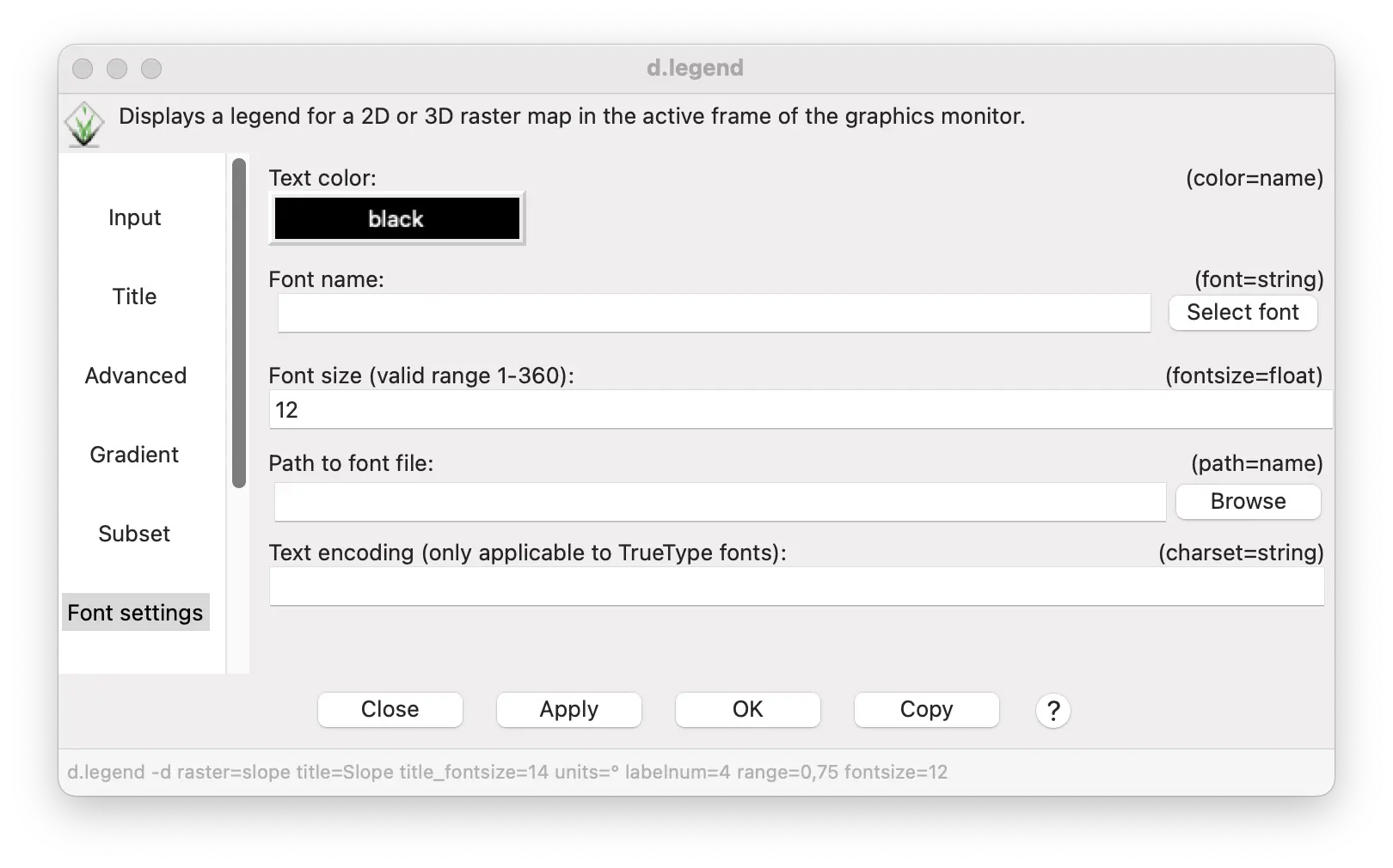
Finally, under the Font settings tab, enter 12 as the “Font size” for the legend.
Click OK to see the legend. You can reposition and resize the legend with a mouse or numerically under the Options tab.
A legend can be generated using the d.legend command.
d.legend -d raster=slope title=Slope title_fontsize=14 units=° labelnum=4 range=0,75 fontsize=12A legend can be generated using the d.legend command.
gs.run_command("d.legend",
map="slope",
color="slope",
title="Slope",
title_fontsize=14,
units="°",
labelnum=4,
range="0,75",
fontsize=12)Here is the result.
It not only shows the range of slope values and colors of different slope values, but also the histogram shows the number of cells for each slope value.
You can also add a scale bar and north arrow from the same menu bar item in the display window where you selected the legend tool.
Displaying specific slope values
Rather than seeing all slopes or other terrain characteristics, it is sometimes useful to focus on a limited range values. This can be done quickly in the display properties tool for raster maps.
Make sure that the slope map and the relief maps are showing in the Layer Manager (Double click a map in the Data Catalog to add it to the Layer Manager). The slope map should be above the relief map.
Double click on the slope map to open its display properties tool. (d.rast)
Under the Selection tab, enter 10-76 to display only slopes at 10° or above, and click Apply or OK.
You can display this over the relief map by setting the opacity to 50%.
You can display only slopes ≥ 10° using the (d.rast) tool.
d.rast map=slope values=10-76You can display only slopes ≥ 10° using the (d.rast) tool.
gs.run_command("d.rast",
map="slope",
values="10-76")Filtering for a limited range of slope values highlights important terrain features of the Flagstaff region.
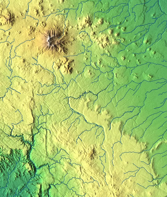
The terrain in this area is dominated by the San Francisco volcanic field, including the San Francisco Peaks strata volcano, and numerous other smaller volcanoes and cinder cones. High slope values accentuate these volcanic features in the upper portion of the map.
At the southwestern corner of the map is the beginning of the Colorado Plateau escarpment, where the land falls rapidly for hundreds of meters into the Rio Verde valley. The deeply incised drainage in this region demarcates this feature of the terrain.
Topographic Landforms
Slope, aspect, and related analyses can help identify terrain features like volcanoes and canyons. GRASS also offers tools to identify topographic features and classify terrain into landform categories. In the standard GRASS tools set, these include:
r.geomorphon: Calculates geomorphons (terrain forms) and associated geometry using machine vision approach.
r.param.scale: Extracts terrain parameters from a DEM.
Additional GRASS Addons useful for this kind of terrain analysis include:
In this tutorial, we will briefly explore r.geomorphon to classify the DEM into a set of landform categories. You are encouraged to try out the other tools for using the standard GRASS sample data sets or your own data.
The r.geomorphon tool identifies and classifies a cell using information about the topographic relief in eight directions (see the r.geomorphon Description for more details)). There are a number of options.
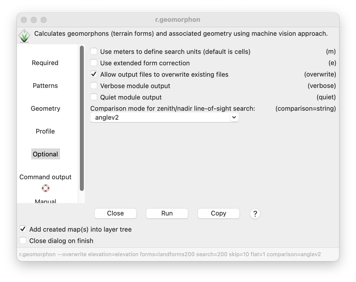
The most important option is the Outer search radius, which is the maximum distance that the algorithm will record topographic relief. By default, this distance is measured in map cells, but you can change it measure in meters with the “-m” option.
When the radius is small, the terrain will be classified into local, small-scale landforms: e.g., small hillocks, gullies, and local depressions. When the radius is large, the terrain will be classified into larger landforms: e.g., large hills and mountains, valleys, basins.
An Inner search radius can be set to have the tool ignore all minor relief near a cell.
We will start with a large outer search radius of 200 cells (6 km on the Flagstaff DEM). This will classify larger scale landforms.
Select the r.geomorphon tool from the Raster/Terrain analysis/Landforms menu.
Enter 200 for “Outer search radius” and 10 for “Inner search radius”.
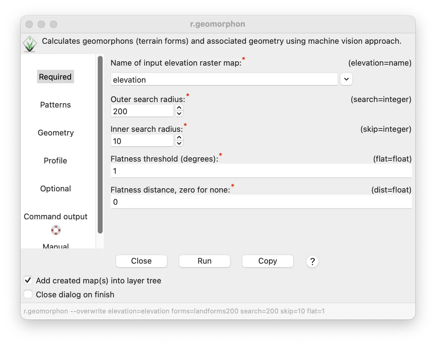
- Enter landforms200 for the output map in the “Most common geomorphic forms” text box.
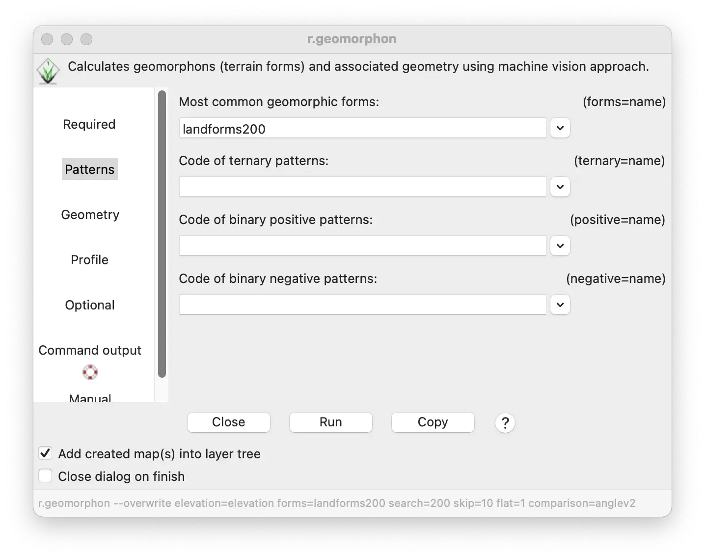
Under the Optional tab, set the “Comparison” to anglev2_distance for better results.
Click Run. This analysis may take a few minutes depending on your processor and RAM.
Now create an analysis of very small landforms using a search radius of only 5 cells (150 m).
- Repeat the same steps for the large landforms but with 5 for “Outer search radius” and 0 for “Inner search radius”. The analysis will run much faster with these settings.
We will start with a large outer search radius of 200 cells (600 m on the Flagstaff DEM). This will classify larger scale landforms.
r.geomorphon elevation=elevation forms=landforms200 search=200 skip=10 flat=1 comparison=anglev2_distanceRepeat with a much smaller search radius to classify much smaller landforms.
r.geomorphon elevation=elevation@terrain forms=landforms5 search=5 skip=0 flat=1 comparison=anglev2_distanceWe will start with a large outer search radius of 200 cells (600 m on the Flagstaff DEM). This will classify larger scale landforms.
gs.run_command("r.geomorphon",
elevation="elevation",
forms="landforms200",
search=200,
skip=10,
flat=1,
comparison="anglev2_distance")Repeat with a much smaller search radius to classify much smaller landforms.
gs.run_command("r.geomorphon",
elevation="elevation",
forms="landforms200",
search=5,
skip=0,
flat=1,
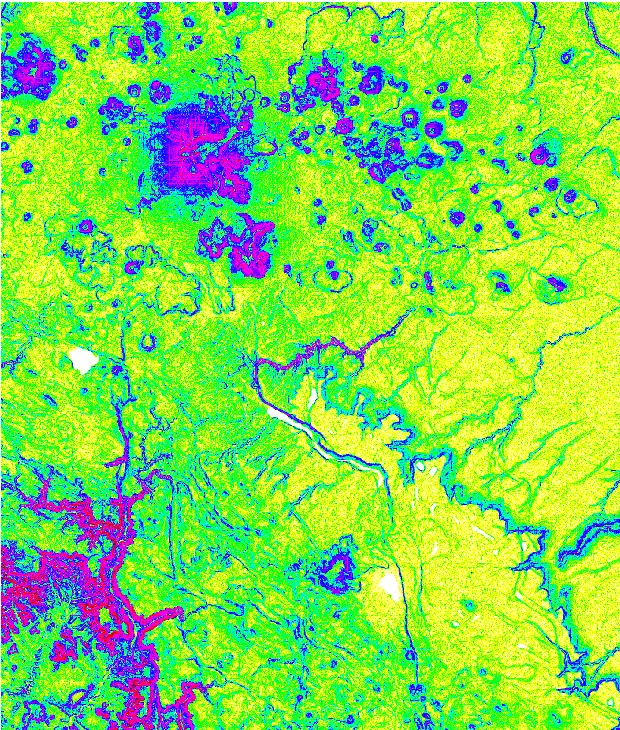
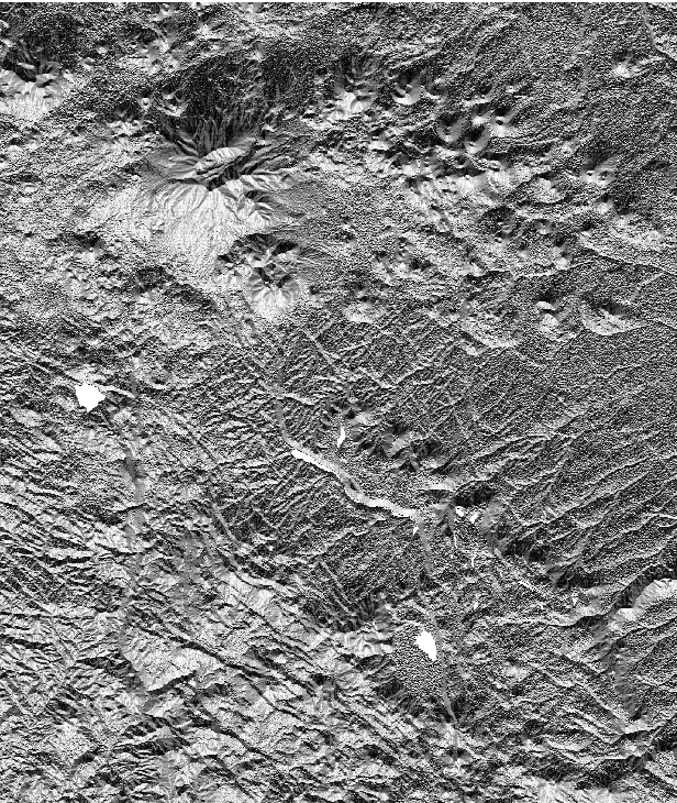
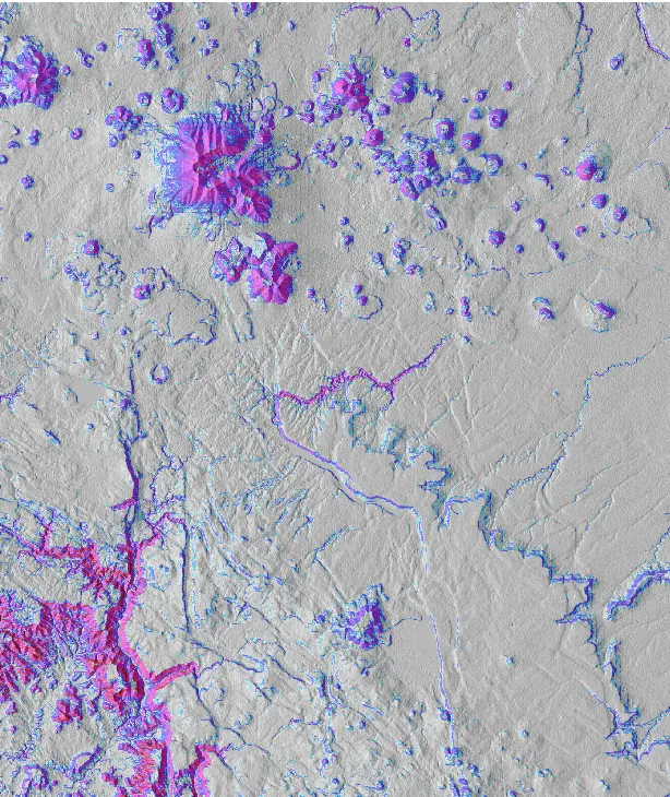
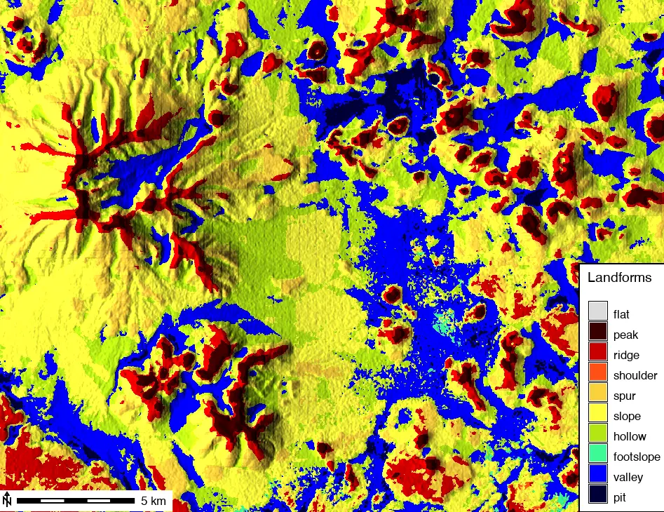
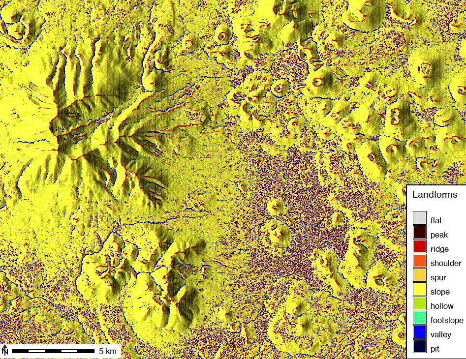
comparison="anglev2_distance")The two images below show landforms classified by r.geomorphon at different scales in a closeup of the Flagstaff elevation DEM focusing on a section of the San Francisco volcanic field. The landforms maps are shown as color shading over the topographic relief map.
At the larger scale (200 cell search radius), peaks and ridges mark the summits of all the large volcanoes and small cinder cones. They are surrounded by zones of spurs, slopes, and hollows, divided by valleys, indicating their lava fields.
At the smaller scale (5 cell search radius), the narrow rims of the volcanic craters are marked by ridges, with crater interiors often demarcated by valleys and pits. The volcanic features are all classified as slopes.
Watersheds and Modeling Hydrology
Because DEM rasters make it possible to generate maps of slope and aspect, this information can be used to model the flow of water across the topographic relief of terrain. This, in turn, permits a wide range of analyses often described as watershed or hydrological modeling. Examples of watershed modeling include:
modeling flow accumulation, representing the quantity of water that passes over each cell as water flows downslope across a terrain;
identification of watershed basins, the portion of a terrain that drains into a stream network of a given size;
modeling a stream or drainage network given the locations of highest flow accumulation within a watershed basin;
modeling potential erosion as a function of the amount of water flowing across cells of a terrain, their slope (affecting the speed of water flow), land cover, and substrate.
modeling the potential for floods;
modeling potential infiltration of surface water and its impact on vegetation and groundwater;
and many other environmental phenomena.
GRASS has many modules for analyzing and modeling hydrology and watersheds, far more than can be covered in this tutorial. Rather, the goal of this tutorial is to give you a sense of what the potential for watershed modeling in GRASS and encourage you to explore its rich array of tools on your own. To that end, this tutorial will explore a few of many features of two of these tools, r.watershed and r.stream.extract.
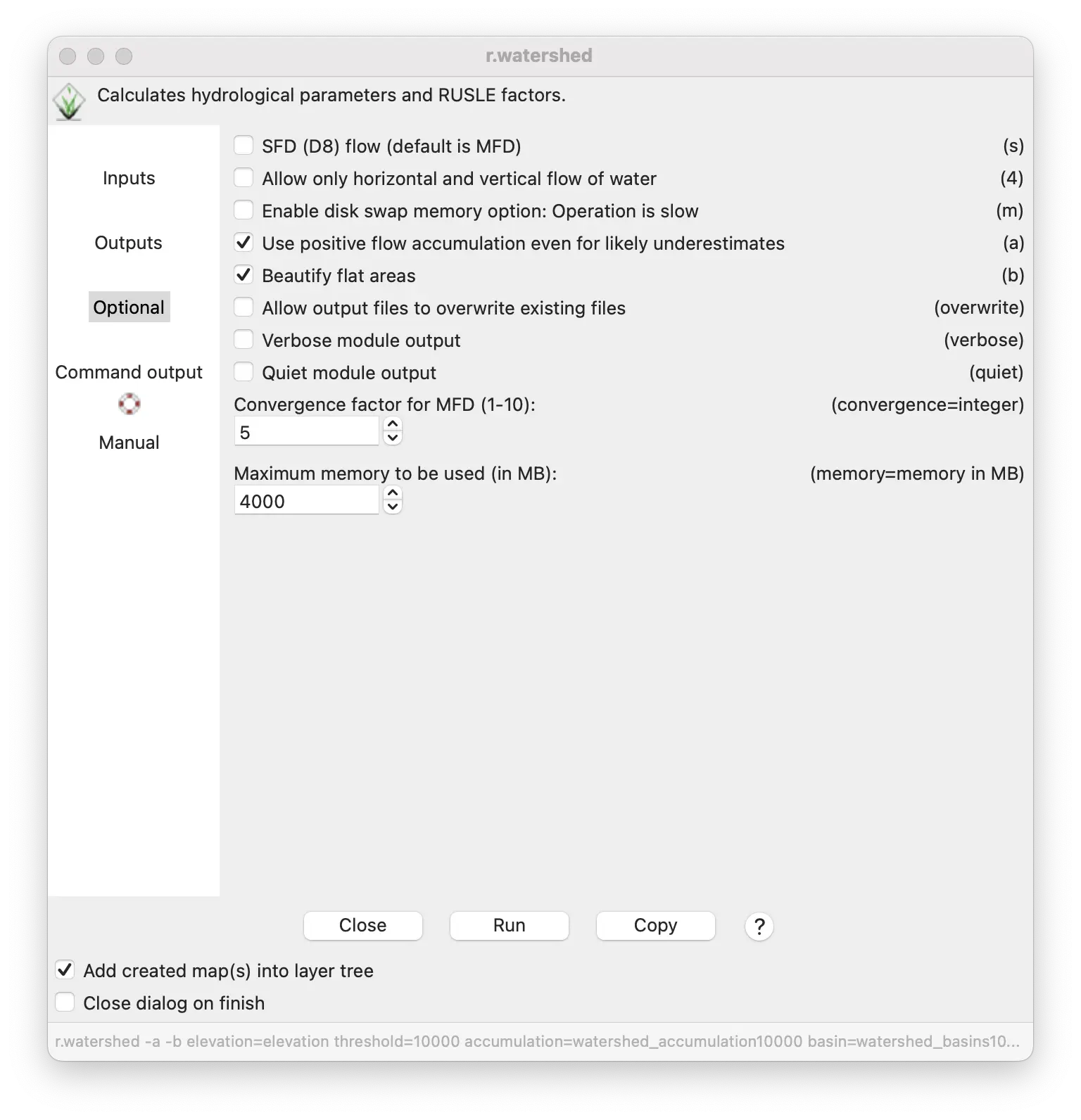
Watershed basins
Watershed basins are portions of a terrain in which all surface water will flow overland and into a single drainage system and exit the basin though a single outlet. They can be as small as a few kilometers or as large as the watersheds encompassing all of the water that flows into the Mississippi or Amazon rivers.
While there are many possible inputs to affect how r.watershed models different hydrological characteristics, we will use the simplest example here.
The minimum required for modeling watershed basins, flow accumulations, and stream networks is a DEM (elevation) and the minimum size of the watershed basins to model (measured in number of cells). We will create basins with a minimum size of 10,000 cells (9 km2). Choosing a smaller number would generate a map of many smaller basins.
Although we start with mapping watershed basins, to save time, we will have r.watershed also generate outputs for flow accumulation and stream segments at the same time it is creating a basin map.
To produce better looking basin and streams maps, we will also select the “Positive flow accumulation” and “Beautify flat areas” options.
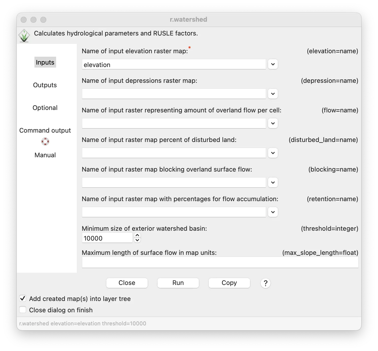
Open the r.watershed module from the Raster/Hydrologic modeling/Watershed analysis menu.
Set “Name of elevation raster map” to elevation.
Enter 10,000 for “Minimum size of exterior watershed basin”.
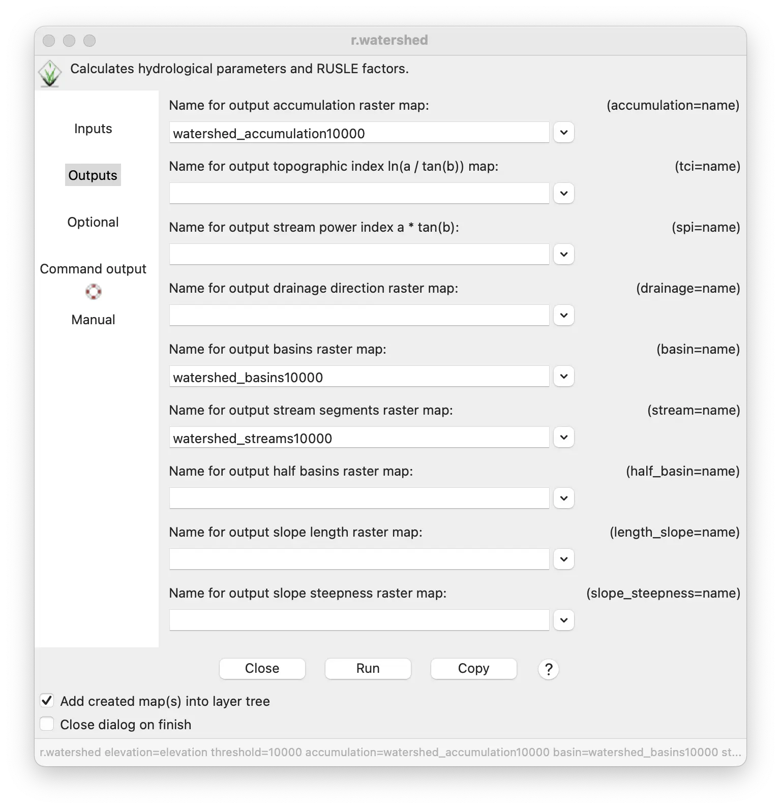
- Under the Outputs tab, enter:
watershed_accumulation10000 for “accumulation”,
watershed_basin10000 for “basins”, and
watershed_streams10000 for “stream segments”.
- Under the Optional tab:
Check the “Positive flow accumulation” box. Otherwise flow accumulation will be negative for basins at the map edge, to indicate that they may under-represent accumulation.
Check the “Beautify flat areas” box to have more accurate stream segments across flat areas.
- Click Run
r.watershed -a -b elevation=elevation threshold=10000 accumulation=watershed_accumulation10000 basin=watershed_basins10000 stream=watershed_streams10000gs.run_command("r.watershed",
elevation="elevation",
threshold=10000,
accumulation=watershed_accumulation10000,
basin="watershed_basin10000",
stream="watershed_streams10000",
flags="ab")Resulting map of watershed basins.
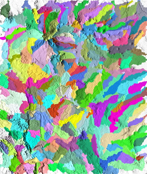
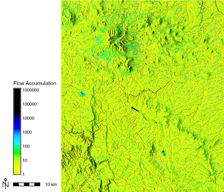
Flow accumulation
Above, we also made a flow accumulation map. A flow accumulation map models the potential flow of water over a terrain:
Assuming a centimeter of rain falls on each cell of a DEM, the values of a flow accumulation map will show the depth of water in centimeters that accumulates and flows over each cell as the water flows into the cell from adjacent upslope cells.
The map we made assumes that the same amount of rain fell on every cell and topographic relief is the only thing affecting overland flow of water. Hence, the flow accumulation model generated represents maximal values.
Additional settings in r.watershed enable modeling overland flow more realistically with different amounts of rain falling across the region, and vegetation, soil characteristics, or barriers like dams or dikes also affecting accumulation.
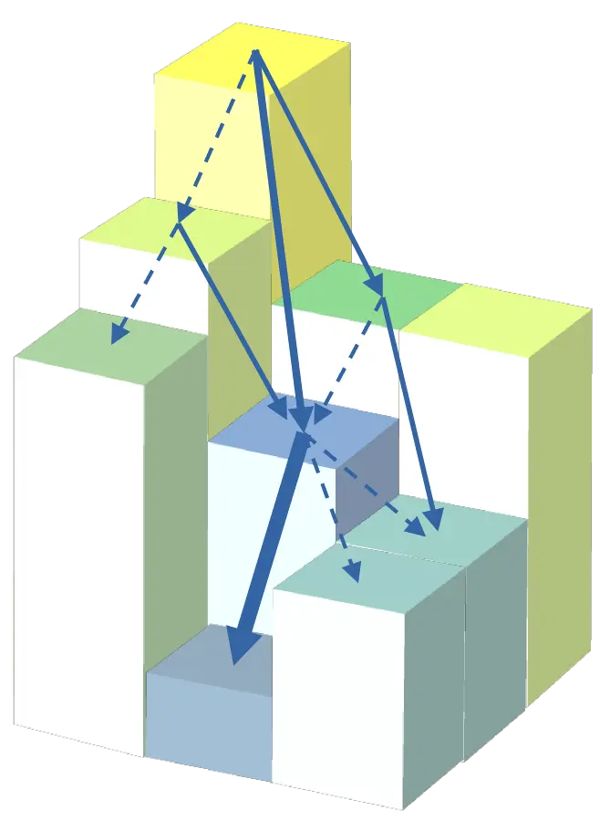
r.watershed uses a multiple flow direction algorithm by default in which water flowing out of a cell is distributed among all adjacent downslope cells. The greatest flow is directed to the adjacent downslope cell with the greatest elevation difference and lower flows are allocated to downslope cells with lesser elevation difference.
While some hydrology modeling tools require depressions or sinks in a DEM to be filled first in order to properly route water across a terrain, r.watershed does not require this. Rather is uses a least cost path algorithm to route water across depressions.
As with slope, a legend can help convey the information of a flow accumulation map more clearly. The distribution of accumulation values is non-linear, however, with many cells on hillslopes having minimal accumulation and a few cells in the bottoms of major streams having much higher values. For this reason, a logarithmic scale better communicates the relationships between colors and values. Create a legend as described previously but with some additional options.
Name of raster map: watershed_accumulation10000@terrain (Input tab).
Legend title: “Flow Accumulation” (Title tab).
Title font size: 14 (Title tab).
Use logarithmic scale: check the box (Advanced tab).
Specific values to draw ticks: 1,10,100,1000,10000,100000,1000000 (Gradient tab).
Font size: 12 (Font settings tab).
d.legend -l raster=watershed_accumulation100000 title="Flow Accumulation" title_fontsize=14 label_values=1,10,100,1000,10000,100000,1000000 fontsize=12gs.run_command("d.legend",
raster="watershed_accumulation10000",
title="Flow Accumulation",
title_fontsize=14,
label_values="1,10,100,1000,10000,100000,1000000",
fontsize=12,
flags="l")Here is a flow accumulation map with a legend using a logarithmic scale. Note higher accumulation on the slopes of the San Francisco peaks, in major stream courses, and in small, shallow lake depressions.
Stream networks
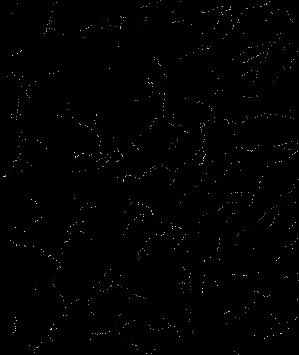
r.watershed also produced a maps of streams, representing the primary drainages of each 10,000-cell watershed basin.
It is a raster map of streams with each stream cell coded and colored to match the basin that it drains, seen in the map of the Flagstaff region to the right.
The background is set to black in the display properties because it is otherwise very difficult to distinguish the raster stream cells.
Vectorizing stream network with r.to.vect
We can make the streams more easily visible if we convert the raster stream map to a vector line map. This can be done easily with the r.to.vect tool that converts rasters maps into vectors.
r.to.vect can convert points, lines, and areas. In this case, we will convert the stream segments created by r.watershed into vector lines.
The raster stream segments are coded with the values of the watershed basins they drain. These values can be transferred to the equivalent vector line segments.
Select the r.to.vect tool from either the Raster/Map type conversions/Raster to vector or the File/Map type conversions/Raster to vector menu.
Enter the map watershed_streams10000 as the “Name of input raster map”.
Enter watershed_streams10000 as the “Name for output vector map”.
Enter line as the “Output feature type”.
Under the optional tab, check the box for “Use raster values as categories instead of unique sequence”. This will copy the basin number into the CAT index key field of the new vector line map.
Click Run.
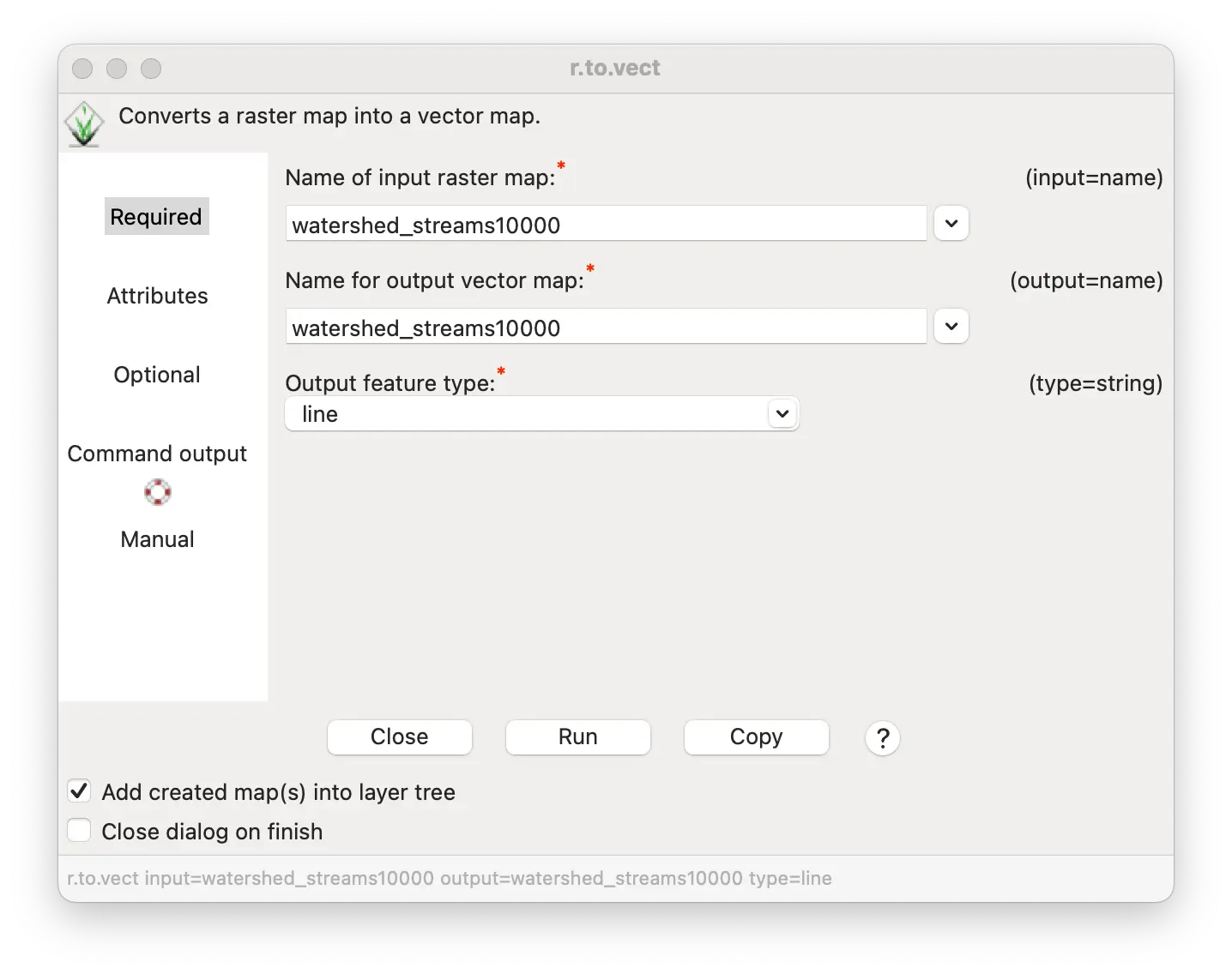
r.to.vect -v input=watershed_streams10000 output=watershed_streams10000 type=linegs.run_command("r.to.vect",
input="watershed_streams10000",
output="watershed_streams10000",
type="line",
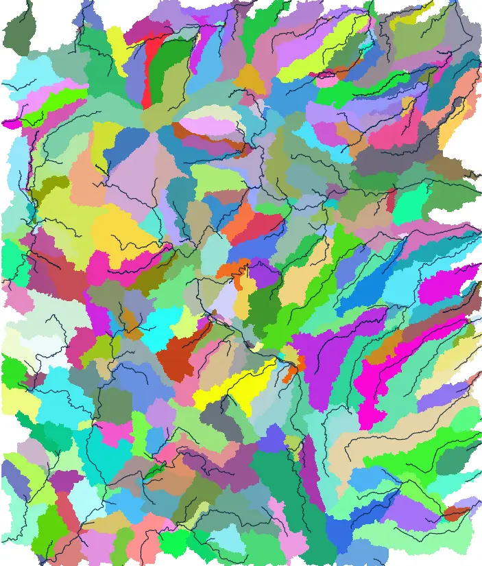
flags="v")The maps below show the vector stream network overlaying watershed basins on the left and overlaying a color shaded relief map on the right.
NoteTip
For a more detailed stream network, run r.watershed with a minimum basin size smaller than the 10,000 cells used above. If you choose a very small minimum basin size to create a very detailed stream map, you may be prompted to run r.thin before running r.to.vect to make sure that raster stream map consists of only single grid cell stream lines.
Vectorizing stream network with r.stream.extract
An alternative way to generate a stream network from a watershed analysis is with the r.stream.extract tool.
This tool uses a DEM and a flow accumulation map to generate a vector or raster stream network.
The detail of the stream network is controlled by selecting the minimum flow accumulation to use.
r.stream.extract not only creates a vector line map of streams, it also generates vector points at the head of each stream and at the junctions of a stream with all other streams.
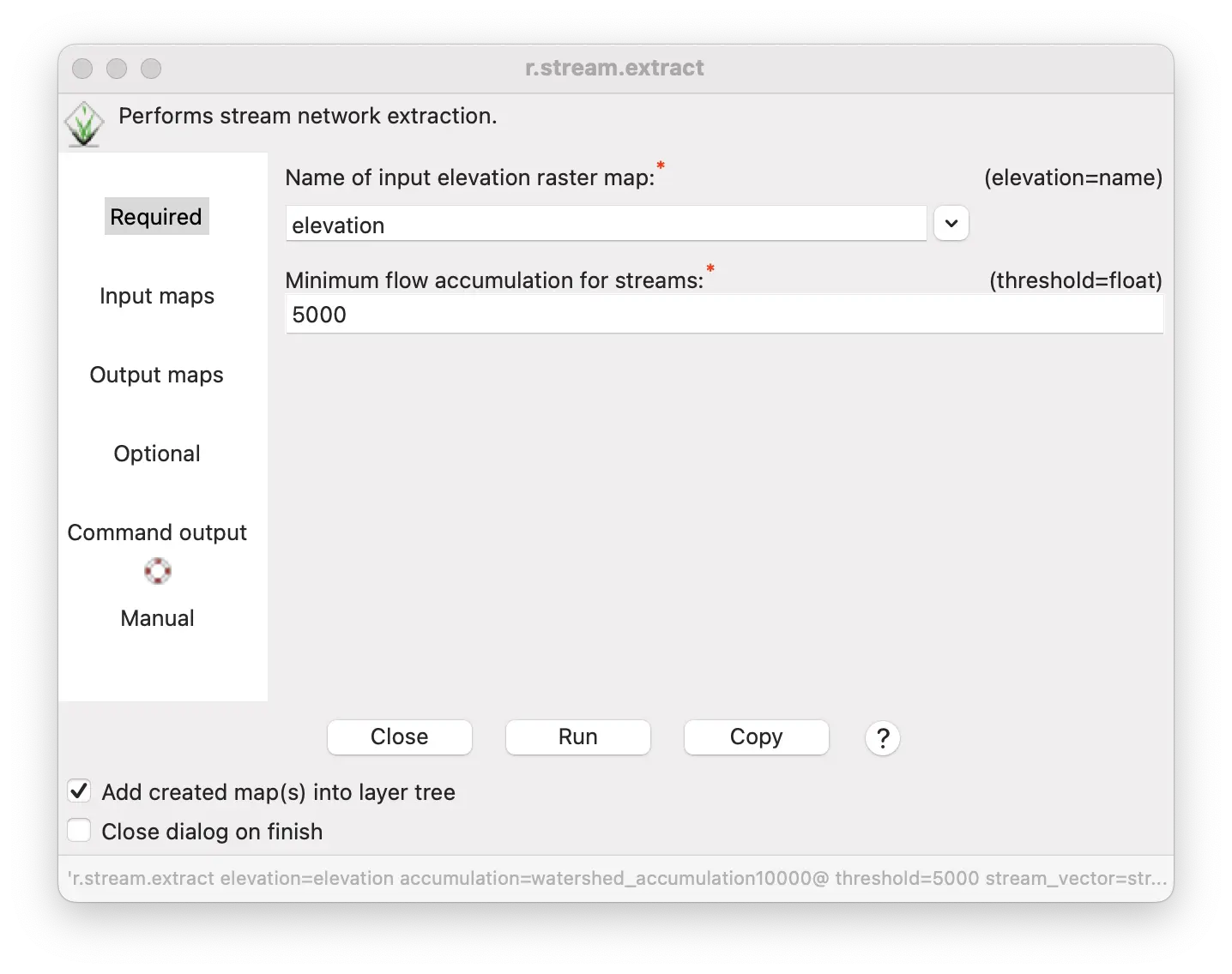
Select the r.stream.extract tool from either the Raster/Hydrologic modeling/Extraction of stream networks menu.
Enter elevation for the “Name of input elevation raster map”.
Enter 5000 for “Minimum flow accumulation for streams” (smaller numbers will generate a more detailed stream network, while larger numbers will generate a less detailed network).
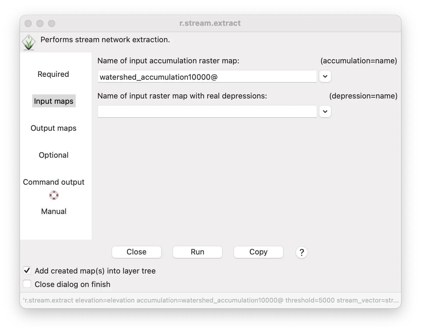
- Enter watershed_accumulation10000 for the “Name of input accumulation raster map”.
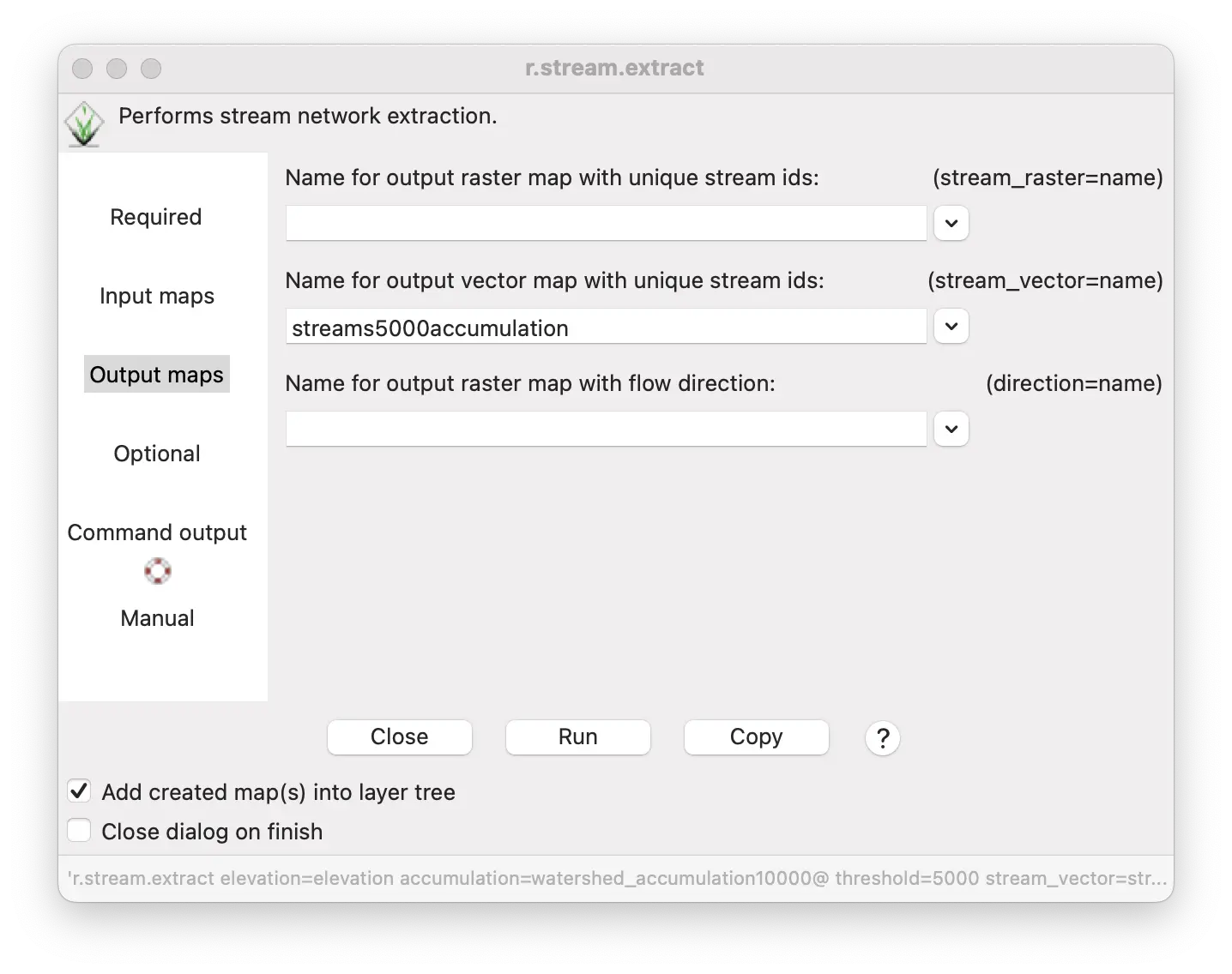
Enter streams5000accumulation for “Name for output vector map with unique stream id”.
Click Run.
r.stream.extract elevation=elevation accumulation=watershed_accumulation10000@ threshold=5000 stream_vector=streams5000accumulationgs.run_command("r.stream.extract",
elevation="elevation",
accumulation="watershed_accumulation10000@",
threshold=5000,
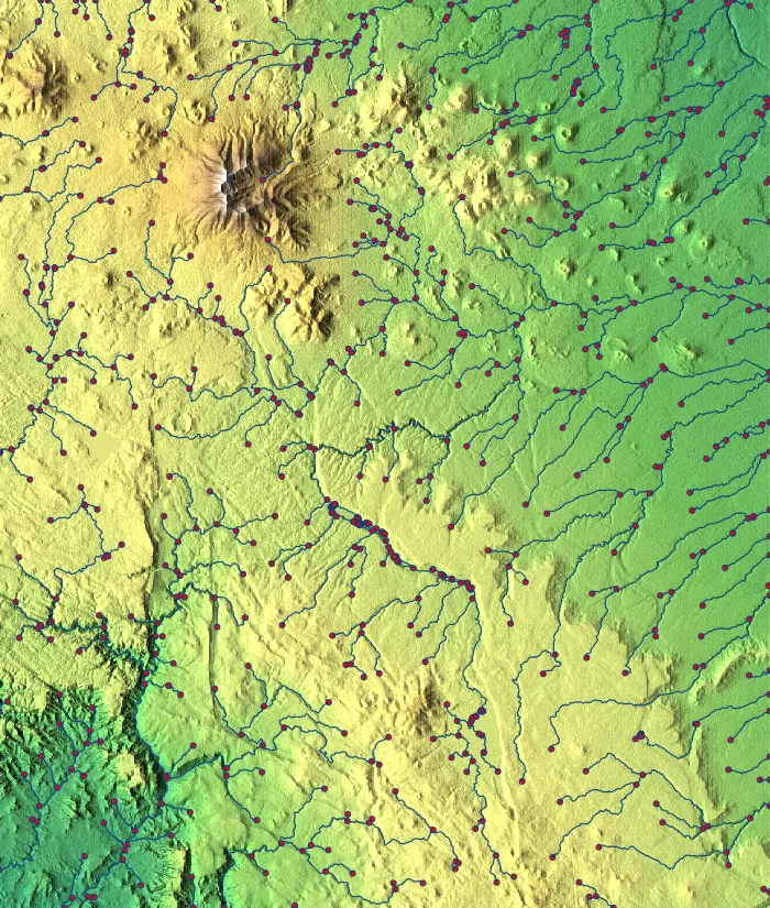
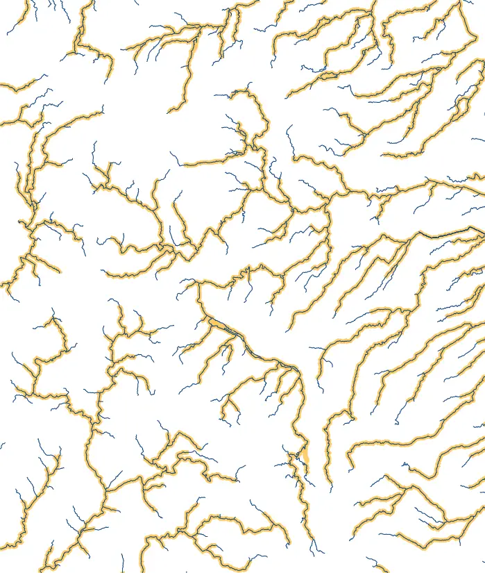
stream_vector="streams5000accumulation")The 2 images below show the stream network generated by r.stream.extract overlaying a color shaded relief map (left) and a comparison of this network with the one generated by r.watershed and then vectorized with r.to.vect (right).
Note the stream lines (blue) and points (red) indicating stream heads and junctions in the left image. Lines or points can be displayed or hidden or shown together in the vector properties tool d.vect.
In the image to the right, the more detailed stream network generated by r.stream.extract is shown in narrow blue lines and the the stream network generated by r.watershed and r.to.vect is shown as wider yellow lines.
NoteTip
To display the stream network without the junction nodes, uncheck the “point” box in the Selection tab of the vector display properties tool (command: d.vect map=streams5000accumulation type=line)
Summary
In this tutorial we have gone over only a few of the many tools available in GRASS to conduct terrain and watershed analysis. We used the Flagstaff sample dataset to complete this analysis, but you can also try this other datasets and DEM maps. You can also use the GRASS sample datasets to explore the many other tools available under the terrain analysis and hydrology hydrology sections. In addition to the main GRASS modules, there are also many others available as GRASS addons.
© Eunice Villaseñor Iribe and Michael Barton 2026 The development of this tutorial was funded in part by the US National Science Foundation (NSF), award 2303651.