Introduction to Remote Sensing with GRASS

Analysis and visualization of multi-band satellite imagery using image fusion, environmental indexes, and dimensionality reduction with principal components analysis.

GRASS has many tools for processing and visualizing remote sensing imagery. This tutorial only scratches the surface of GRASS’s extensive capacity for image processing.

Hopefully, it will give you some sense of the potential for analysis and visualization of remote sensing imagery in GRASS and the potential to combine remote sensing analysis with raster and vector GIS processing.

We will start with a quick overview of multi-band satellite imagery.

Landsat 8 OLI image of the Flagstaff, AZ region. RGB image fusion of bands 3, 4, & 5

Dataset

This tutorial uses one of the standard GRASS sample data sets for Flagstaff, Arizona, USA: flagstaff_arizona_usa. We will refer to place names in that data set, but it can be completed with any of the standard sample data sets for any region–for example, the North Carolina data set.

We will use a set of images from the Landsat 8 satellite and the elevation DEM raster map. However, this tutorial can also be used with other multi-band imagery, such as Sentinel or Terra/ASTER. With other satellite imagery than Landsat 8, the band numbers may differ from those described in this tutorial.

GRASS environment

This tutorial is designed so that you can complete it using the GRASS GUI, GRASS commands from the console or terminal, or using GRASS commands in a Jupyter Notebook environment.

Don’t know how to get started?

If you are not sure how to get started with GRASS using its graphical user interface or using Python, checkout the tutorials Get started with GRASS GUI and Get started with GRASS & Python in Jupyter Notebooks.

Remote sensing basics

Many Forms of Remote Sensing

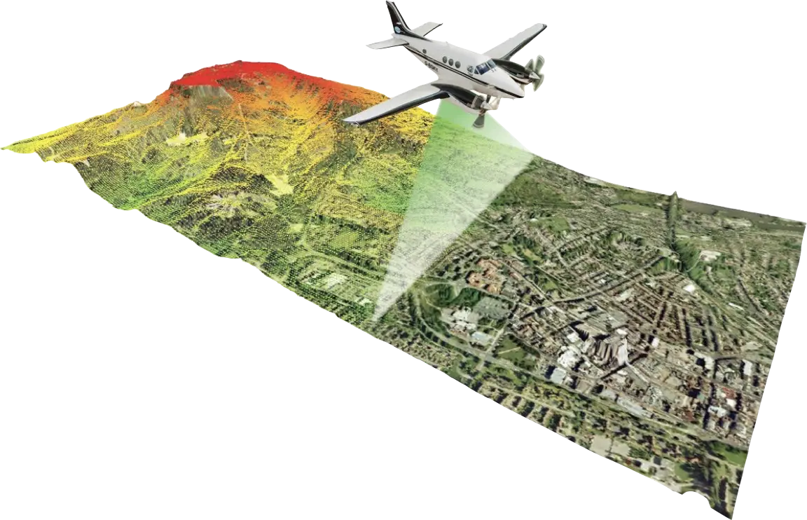
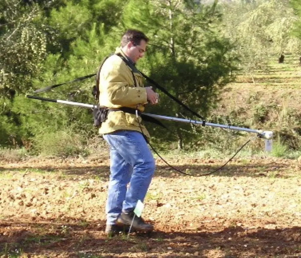
There are many forms of remote sensing. This tutorial will focus on space-based remote sensing platforms.

Space-based platforms (NASA 2015)

Aerial photography and LiDAR

Geophysical survey (© Michael Barton 2025)

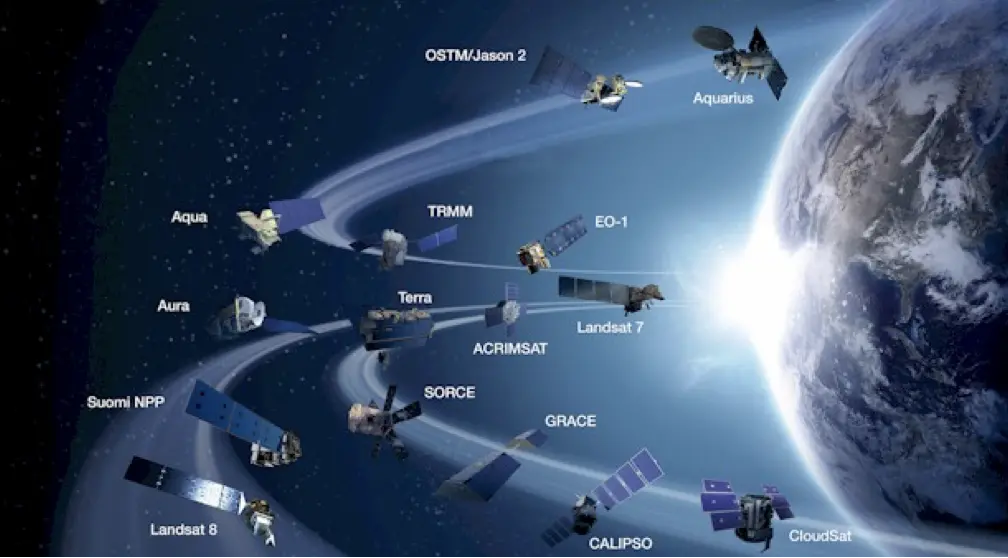
Space-based platforms

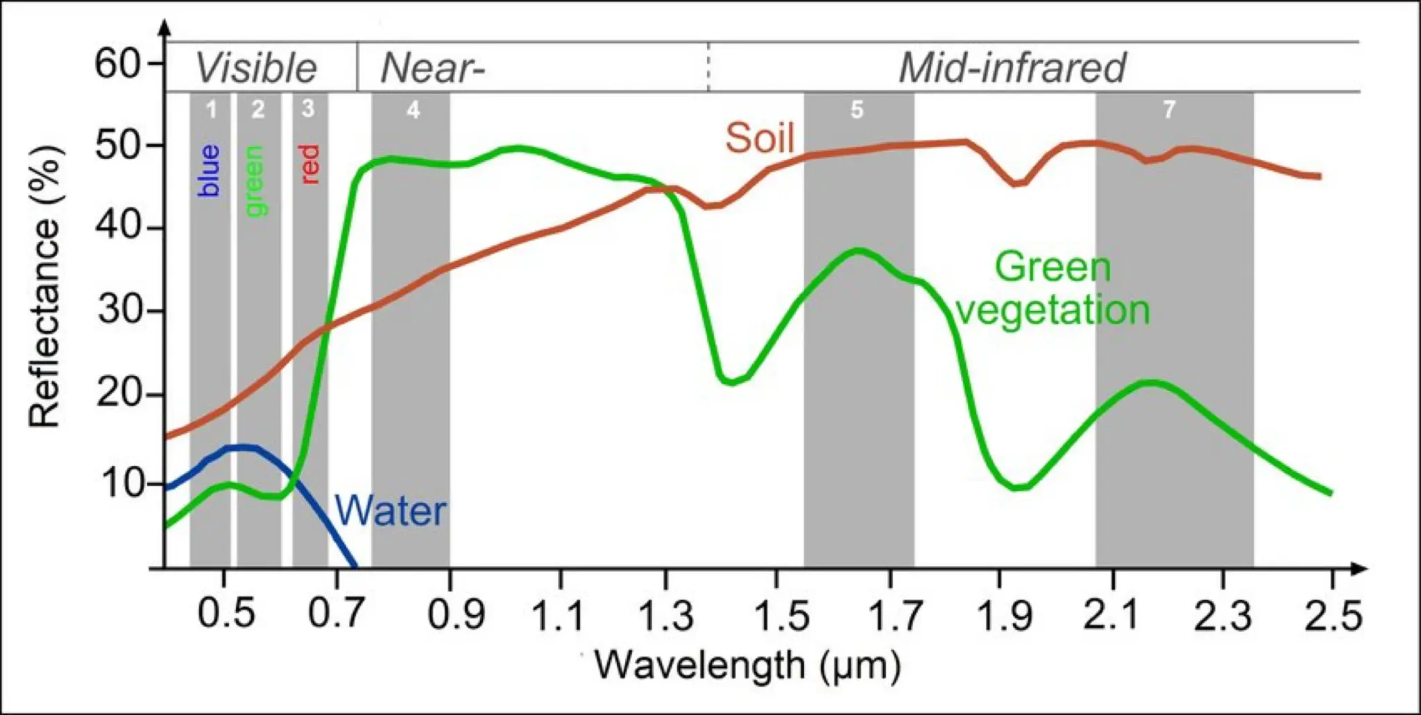
• These satellites have sensors to capture the reflectance of solar electromagnetic (EM) radiation that reaches the earth–including the EM we see as visible light.

• Different materials absorb, emit, and reflect EM radiation in different frequencies.

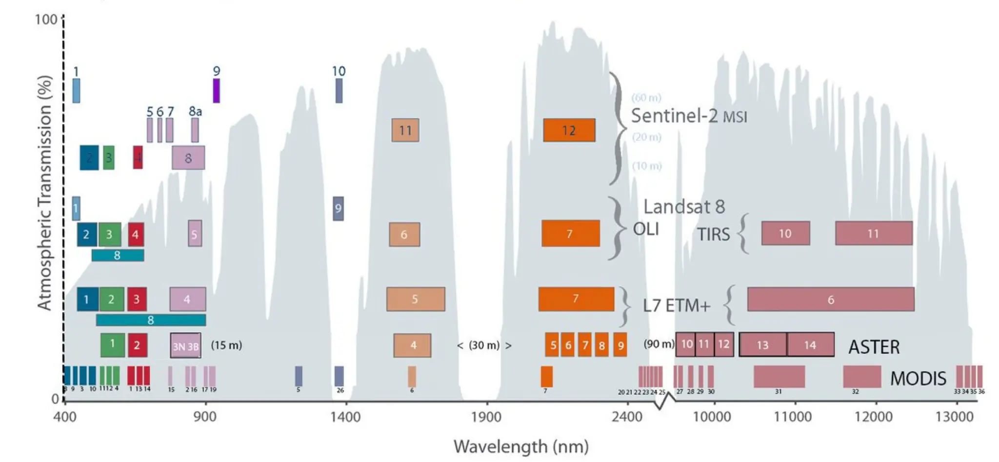
• Space based sensors capture images across multiple EM frequencies in different “bands” or “channels” to enable the identification of different materials or features.

• Sensor band images as rasters can be combined mathematically in different ways to enable visualization or identification of features or materials.

EM reflectance of different materials. Image based on SEOS, Science Education through Earth Observation for High Schools (SEOS), CC BY-NC-SA 2.0.

Image bands of different space-based platforms and EM frequencies that reach the Earth’s surface. Image by L. Rocchio and J. Barsi, NASA

Visualization of multi-band remote sensing imagery in GRASS

GRASS has many tools for combining and analyzing single and multi-band imagery. In this tutorial, we will explore a few of these analytical tools using images of the Flagstaff region from the Landsat 8 satellite.

Landsat 8 image by Robert Simmon, USGS and NASA 2013

Landsat bands to analyze

The following Landsat 8 bands are provided with the Flagstaff data set:

• landsat8_2024_B1 : high frequency visible blue for cirrus clouds
  
• landsat8_2024_B2 : visible blue
  
• landsat8_2024_B3 : visible green
  
• landsat8_2024_B4 : visible red
  
• landsat8_2024_B5 : near infrared
  
• landsat8_2024_B6 : mid infrared (higher freq)
  
• landsat8_2024_B7 : mid infrared (lower freq)

In this tutorial, we will use Landsat 8 bands 2-7.

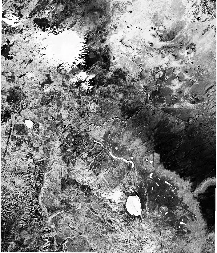
Visualize individual Landsat bands

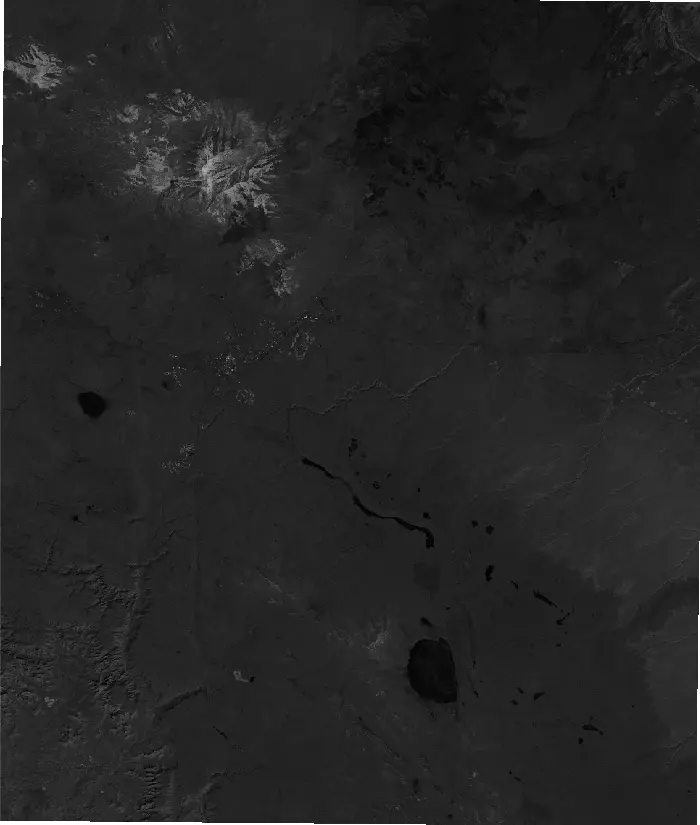
• Load bands 2-7 into the layer manager but not band 1 (landsat8_2024_B1).

• Notice how dark each of the images is.

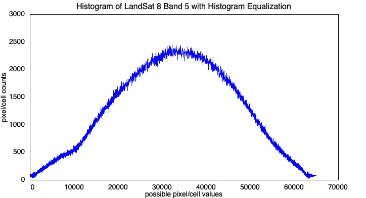
• That is because, although each cell could be one of 65,536 values, nearly all are within a very narrow range.

Histogram of the number of pixels for each possible value

Landsat band 5

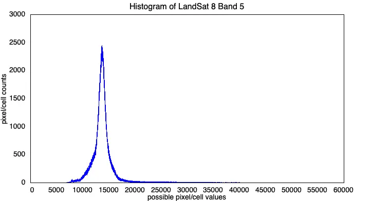
Histogram equalization

The range of grey shades can be remapped across the cell values, so that they fully span a black to white continuum. This can be done in r.colors by “equalizing” the color histogram of the cells.

Distribution of pixel values after histogram equalization

Histogram equalization in GRASS

Using r.colors for histogram equalization will enhance the visibility of the image but will not change its cell values.

GUI

1. Select r.colors from the Raster/Manage colors menu

2. Enter a Landsat image in the Name of the raster map(s) text box

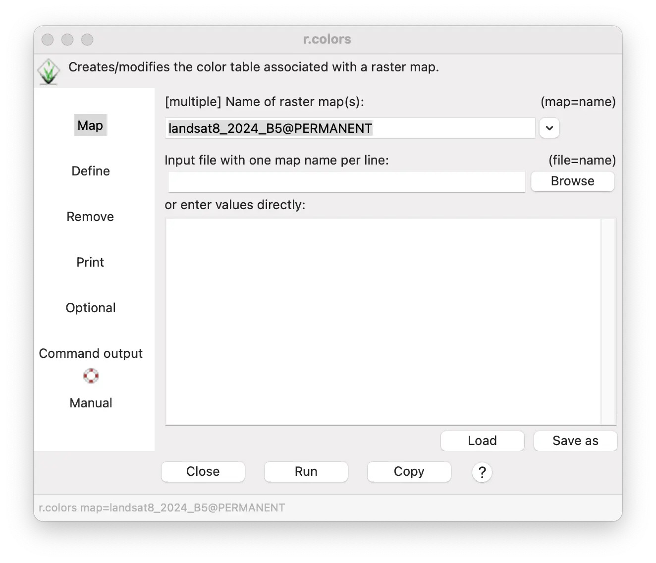
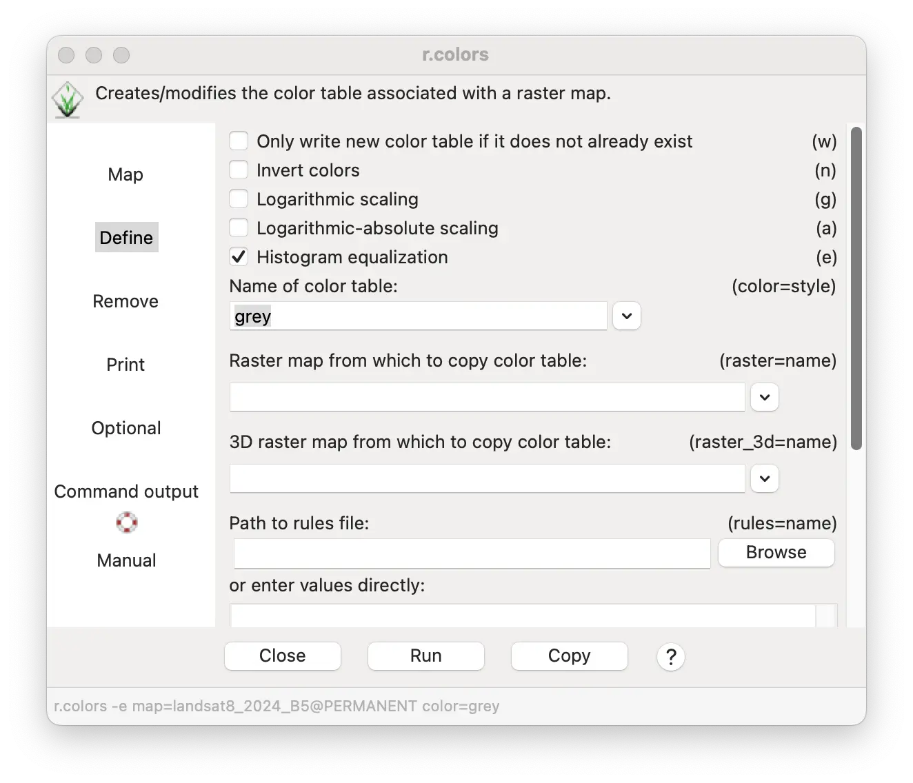
3. Check the histogram equalization box

4. Select grey in the Name of color table text box

5. Press Run

6. Do the same for each of the Landsat bands.

Command line

r.colors -e map=landsat8_2024_B2 color=grey
r.colors -e map=landsat8_2024_B3 color=grey
r.colors -e map=landsat8_2024_B4 color=grey
r.colors -e map=landsat8_2024_B5 color=grey
r.colors -e map=landsat8_2024_B6 color=grey
r.colors -e map=landsat8_2024_B7 color=grey

Python

gs.run_command("r.colors",
               map=landsat8_2024_B2,
               color=grey,
               flags="e")
gs.run_command("r.colors",
               map=landsat8_2024_B3,
               color=grey,
               flags="e")
gs.run_command("r.colors",
               map=landsat8_2024_B4,
               color=grey,
               flags="e")
gs.run_command("r.colors",
               map=landsat8_2024_B5,
               color=grey,
               flags="e")
gs.run_command("r.colors",
               map=landsat8_2024_B6,
               color=grey,
               flags="e")
gs.run_command("r.colors",
               map=landsat8_2024_B7,
               color=grey,
               flags="e")

All examples described in the rest of this tutorial are done with histogram stretched images.

Tip

Histogram each image separately instead of doing all of them together as a group because each image has a different distribution of pixel/cell values to stretch.

---

Landsat band 5 after histogram equalization

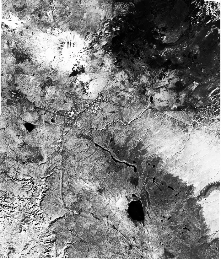
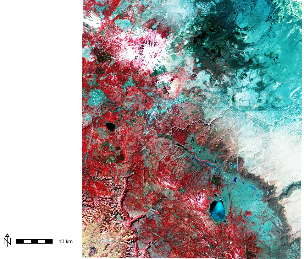
Image fusion

Color image fusion of Landsat bands

Each Landsat image has cell values representing the reflectance intensity in a particular range of EM frequencies (i.e., multiple image bands). When visualized as a raster, a single Landsat band appears as variable, single color (e.g., grey-scale) map.

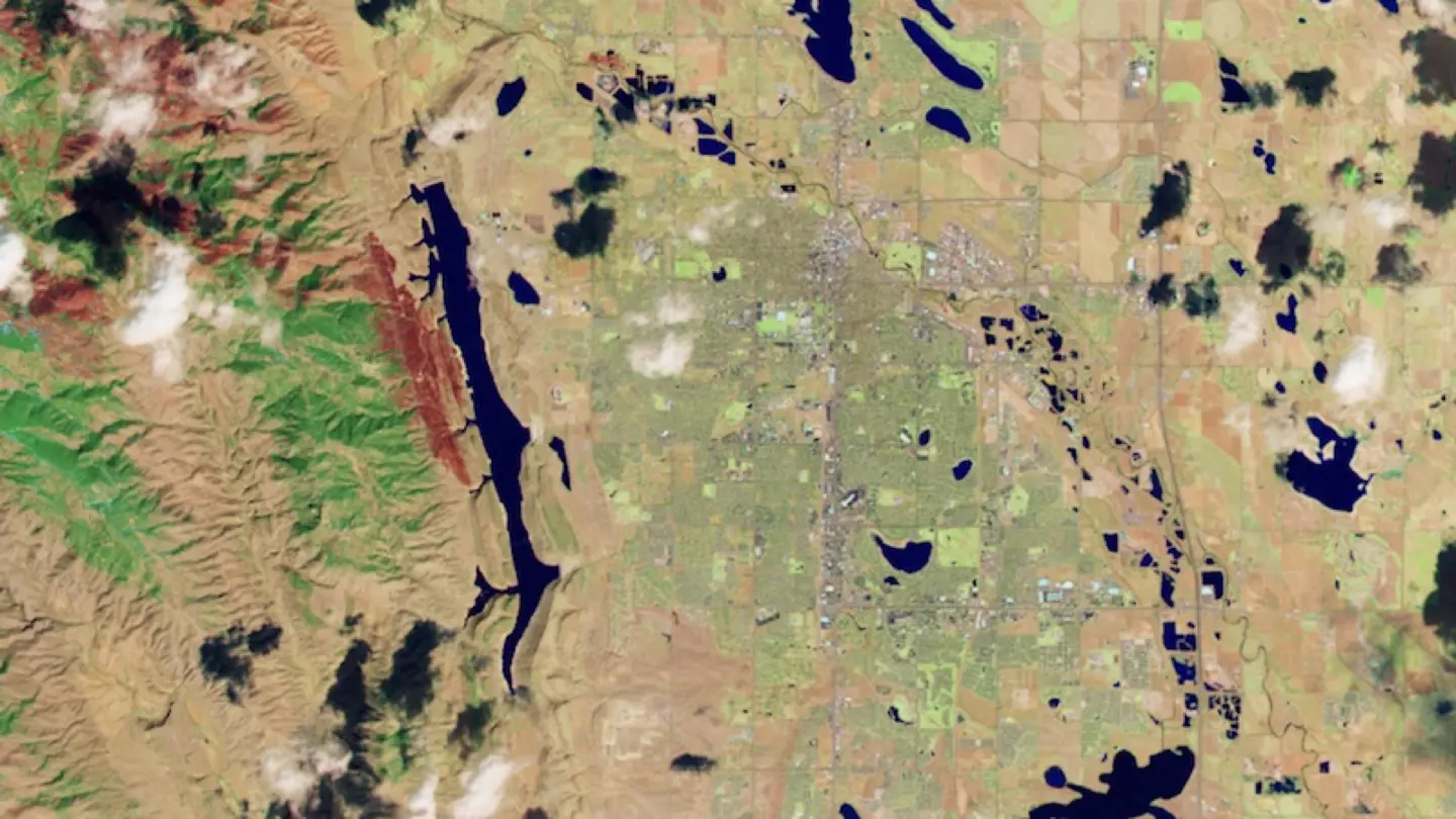
Image fusion refers ways of combining multiple bands in order to visualize them as a full color image. Most simply, this involves defining 3 image bands as the red, green, and blue channels of a multicolor RGB image.. The resulting color visualization displays areas with similar combinations of reflectance across the 3 selected bands (e.g., vegetation, water, or highways) as having the same color and differing from areas with different combinations of reflectance.

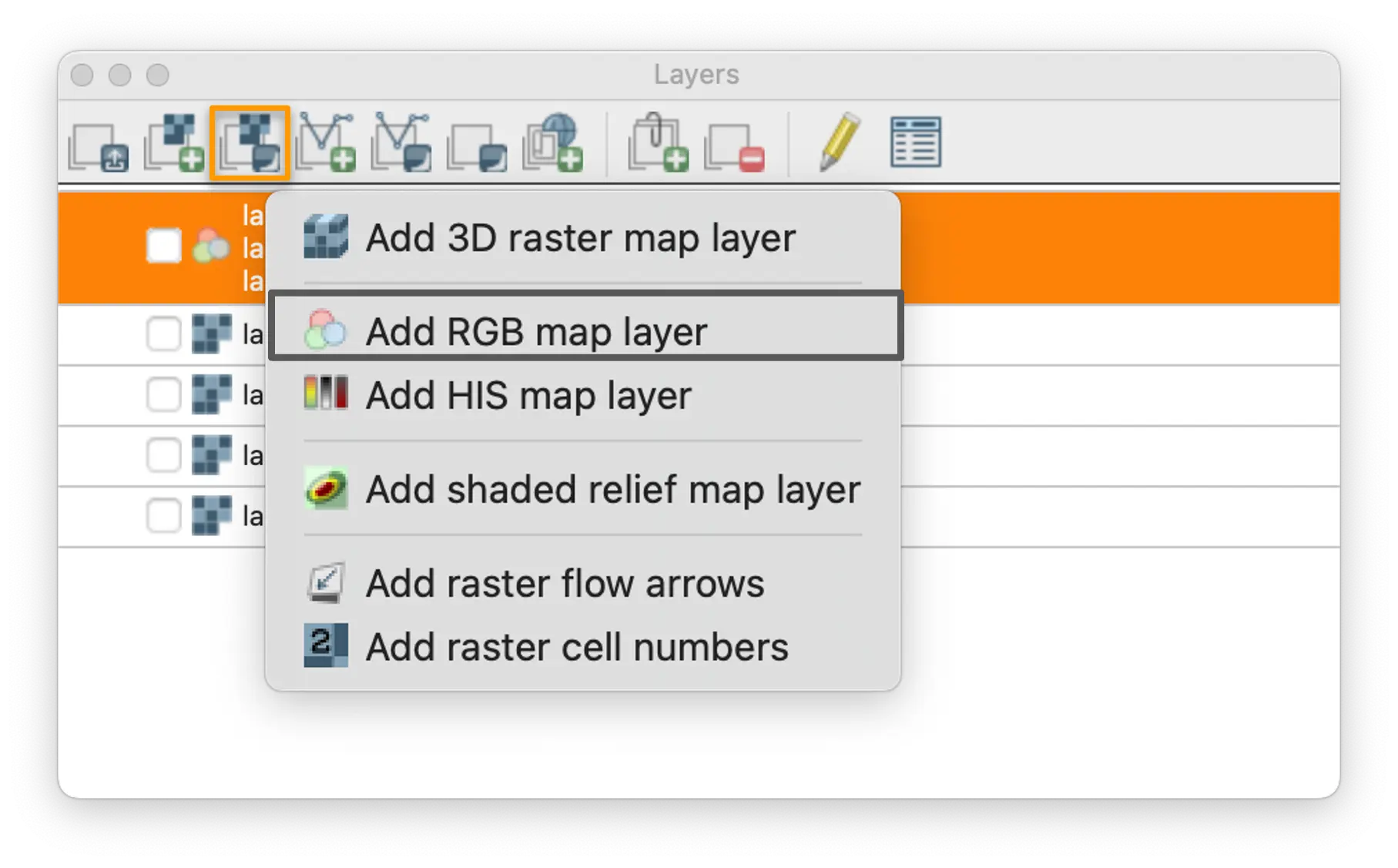
This can be easily done in GRASS using the d.rgb tool in the layer manager.

Image fusion in the layer manager

1. Select Add RGB map layer from the Add various raster layers tool

2. Select Landsat bands to define as the red, green, and blue channels of a multicolor image.

3. For a “natural color” image fusion, try:

   • Band 4 (visible red EM) as red
   • Band 3 (visible green EM) as green
   • Band 2 (visible blue EM) as blue

Natural color image from fusion of Landsat bands 4, 3, & 2

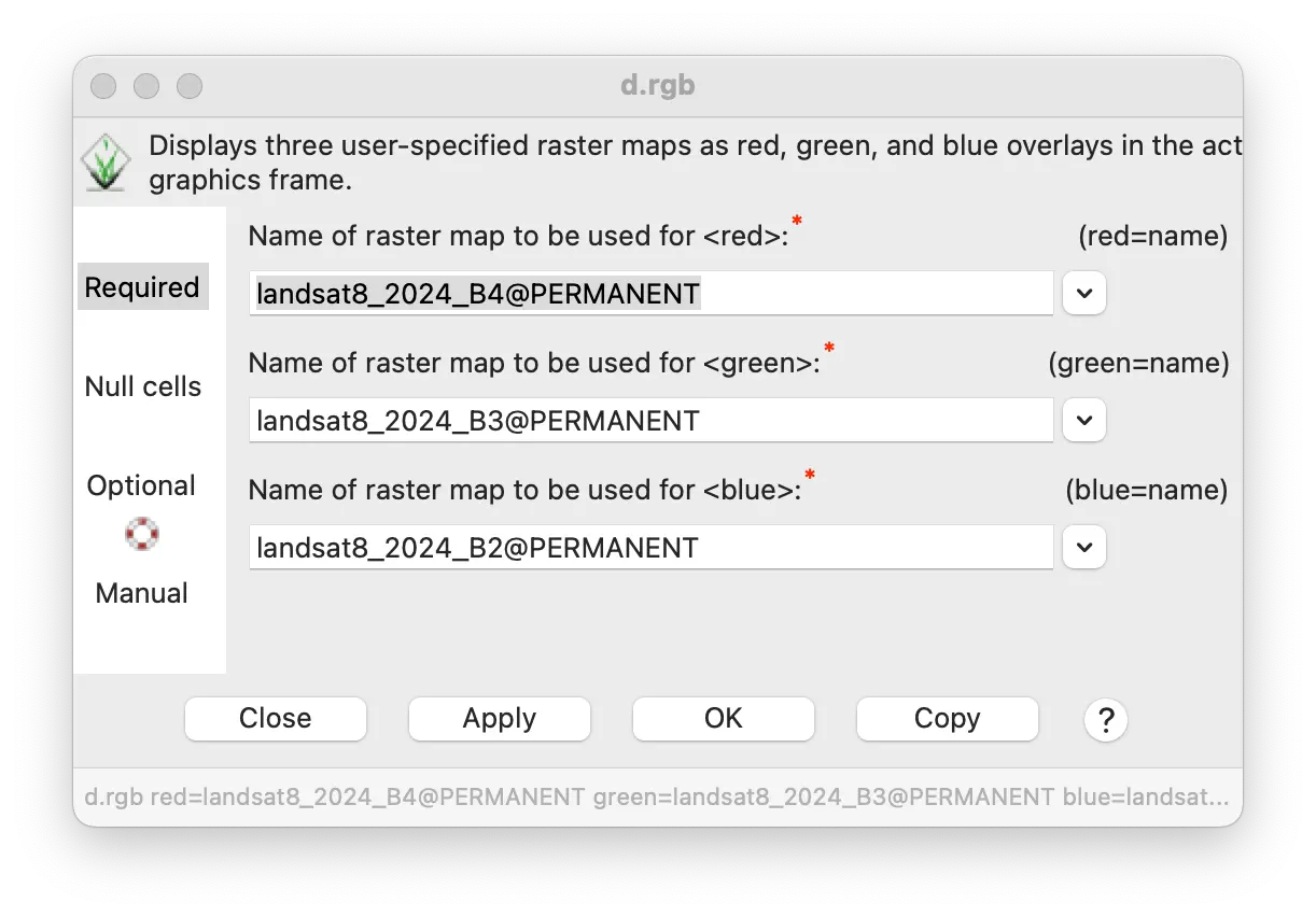
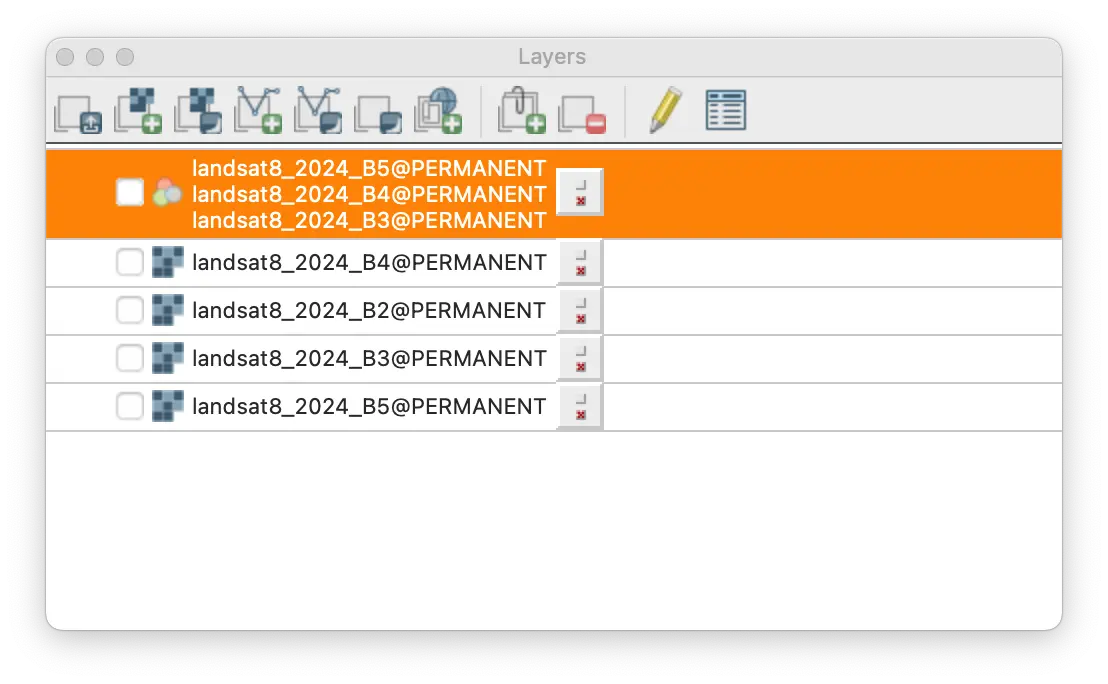
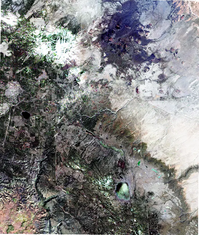
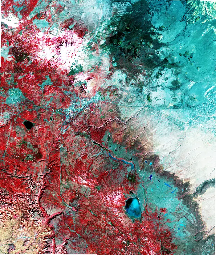
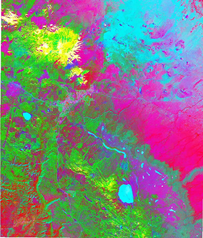
Image fusion: other band combinations

Try some other combinations to highlight different features.

• Using bands 5, 4, and 3 highlights chlorophyll (vegetation) in red.

RGB image from bands 5,4,2

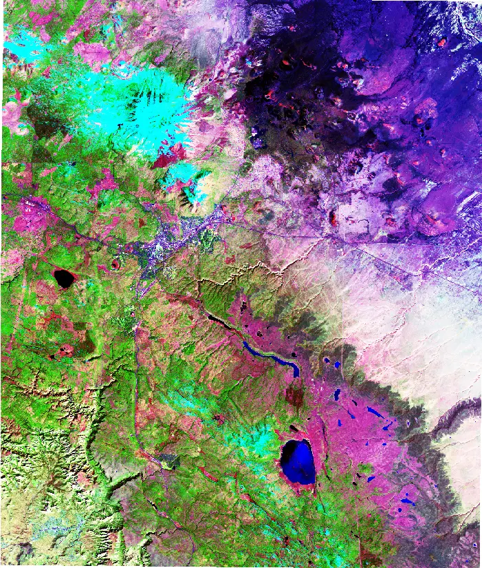
• Image fusion with bands 6, 5, and 3 uses infrared EM to highlight other land cover and land use differently.

RGB image from bands 6,5,2

Environmental indices

Environmental information from mathematical combinations of remote sensing bands

Because different materials—including different vegetation, soils, and water—reflect, absorb, and emit EM in different frequencies, many kinds of environmental information can be derived with different band combinations.

GRASS can generate a large number of environmental indices with its extensive suite of imagery tools (See the Imagery menu), as well as with the raster map calculator. Additional remote sensing image product tools are available as GRASS addon extensions.

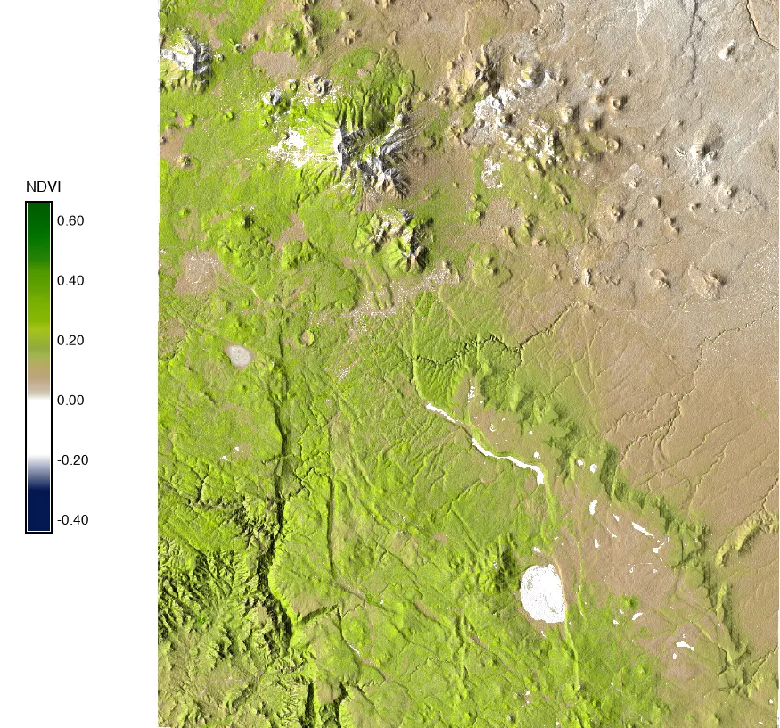
A commonly used environmental index is NDVI : the normalized difference vegetation index. NDVI is an index of plant growth and health. It is computed from bands sensing near infrared (NIR) and visible red light.

\[ NDVI = \frac{NIR - red}{NIR + red} \]

While you could create a map of NDVI using the map calculator, it can also be generated automatically from the GRASS i.vi module, along with many other vegetation indexes.

Tip

When generating any new map, like NDVI, remember to first make sure that the region is set to match the LandSat images

NDVI example: normalized difference vegetation index

GUI

Set the region to match the Landsat images**

1. Add one of the LandSat images raster to the Layer Manager.

2. Right click on the LandSat image in Layer Manager.

3. Select Set computational region from selected map.

Compute NDVI raster

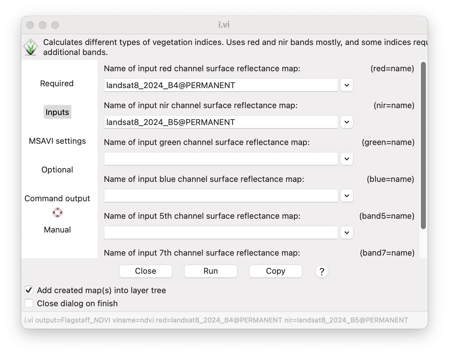
1. Select the i.vi tool from Imagery/Satellite image products/vegetation indices menu.

2. Choose NDVI for the index to calculate

3. Enter the name of the output map to create
   

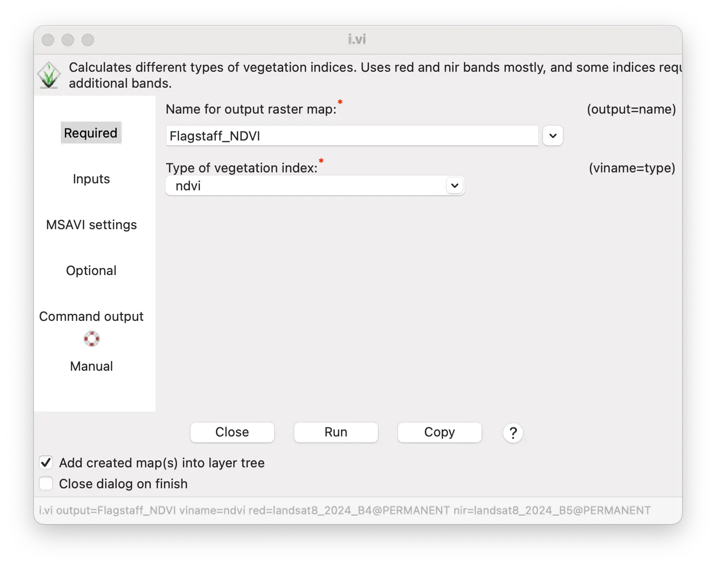
4. Enter band 4 for the red channel

5. Enter band 5 for the NIR (near infrared) channel

Command line

1. Set the region to match the Landsat images

2. Use the i.vi tool to create a map of NDVI values.

g.region raster=landsat8_2024_B2

i.vi output=Flagstaff_NDVI viname=ndvi red=landsat8_2024_B4 nir=landsat8_2024_B5

Python

1. Set the region to match the Landsat images

2. Use the i.vi tool to create a map of NDVI values.

gs.run_command("g.region", raster="landsat8_2024_B2")

gs.run_command("i.vi", 
                output=Flagstaff_NDVI, 
                viname=ndvi, 
                red=landsat8_2024_B4, 
                nir=landsat8_2024_B5
  )

NDVI map shading a relief map of DEM topography

Combining information from many imagery bands

We can visualize 3 bands at a time with RGB color image. But how can we use information from all 6 Landsat bands at the same time? This requires using multivariate statistics for “dimensionality reduction”. GRASS has multiple analytical tools for dimensionality reduction.

Here, we will explore principal components analysis (PCA). PCA mathematically combines the original variables (the Landsat bands) to create new “component” variables that capture majority of variation in original Landsat bands.

PCA of multiband images with GRASS

GUI

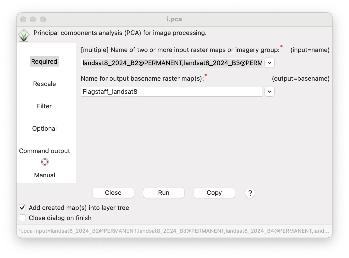
1. Open the principal components analysis (PCA) module, i.pca, found under the Imagery/Transform images menu.

2. Enter names of images for Landsat bands 2-7

3. Provide an output base name. A number, representing the computed PCA component maps will be appended to this output base name.

4. There are other options but the default is OK for now.

5. Press run.

Command line

1. Perform a PCA and output the results to the console/terminal and as PCA component maps

i.pca input=landsat8_2024_B2,landsat8_2024_B3,landsat8_2024_B4, landsat8_2024_B5,landsat8_2024_B6,landsat8_2024_B7 output=Flagstaff_landsat8

Python

1. Perform a PCA and output the results to the console/terminal and as PCA component maps

gs.run_command("i.pca", 
                input="landsat8_2024_B2,landsat8_2024_B3,landsat8_2024_B4, landsat8_2024_B5,landsat8_2024_B6,landsat8_2024_B7", 
                output=Flagstaff_landsat8)

Working with PCA results

Statistical details of PCA output appear in the console or terminal as shown below. Each line of the output represents a PCA component.

The list of values in parentheses is the eigenvector of each PCA component, with the 6 values indicating the contribution of each of Landsat images 2-7 to the component. Larger positive or negative numbers indicate greater contributions of a band to the component. For example, Landsat band 4 has the largest contribution to PCA component 1, while band 6 has the largest contribution to component 2.

The percentage in brackets represent the amount of variation in the original Landsat bands 2-7 are captured by that PCA component. For example, PCA component 1 captures 58% of the variation in the original 6 bands and PCA component 2 captures 35% of the variation.

Eigen values (vectors) [% importance]

PC1 14640530.56 ( 0.4461, 0.4915, 0.5480, 0.4167, 0.1994, 0.2136) [58.03%]
PC2 8850161.06 ( 0.2240, 0.1951, 0.1050, 0.0543,-0.7001,-0.6385) [35.08%]
PC3 1502032.84 ( 0.2335, 0.1528, 0.2947,-0.8794,-0.1102, 0.2231) [ 5.95%]
PC4 108422.28 ( 0.4370,-0.8041, 0.3529, 0.0416, 0.1120,-0.1536) [ 0.43%]
PC5 94291.01 ( 0.4417, 0.2122,-0.4285,-0.1814, 0.5597,-0.4797) [ 0.37%]
PC6 34241.78 ( 0.5570,-0.0735,-0.5418, 0.1242,-0.3636, 0.4931) [ 0.14%]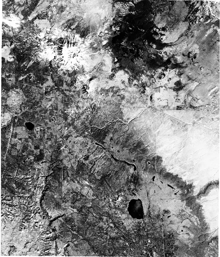

PCA 1 image

PCA 2 image

Visualizing PCA results

To better see spatial variation in a PCA component image, you can assign a different color table from the standard grey-scale. This is often called a “false color image”.

Here is PCA component 1 colored with a bcyr (blue-cyan-yellow-red) color table with histogram equalization checked.

Follow the instructions given above for histogram equalization, but pick bcyr instead of grey for the color table.

Note how areas of different vegetation, soil, and water stand out more clearly than with grey-scale. Try other color tables.

False color image of PCA component 1 of LandSat 8 bands 2-7

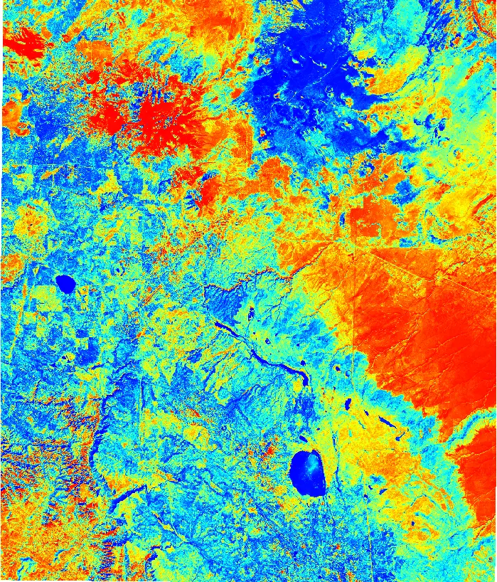
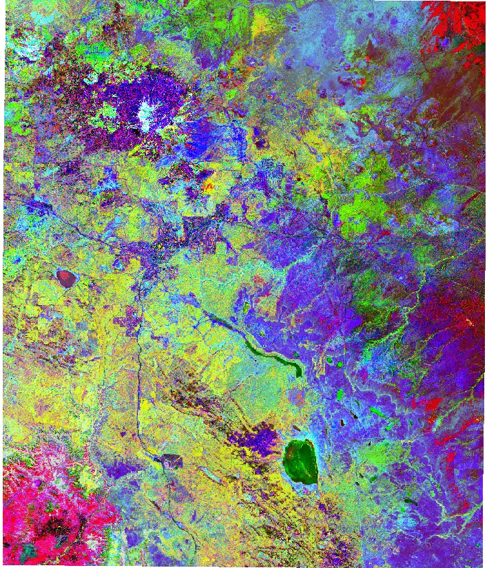
Image fusion with PCA results

The image fusion methods described above for multiple Landsat bands can also be used for PCA results.

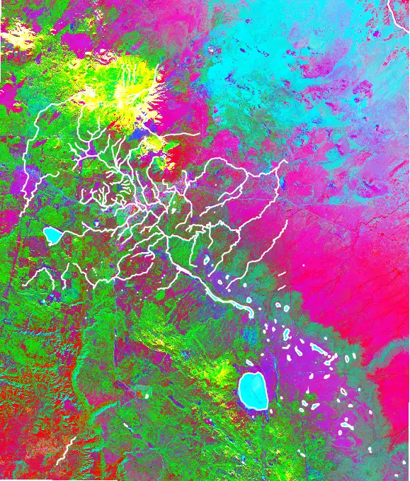
The PCA text output shown above indicates that the first 3 PCA components capture 97% of the variation in the original 6 Landsat bands 2-7. This means that we can visualize nearly all of the information in the original 6 Landsat bands by creating an RGB color image of PCA components 1, 2, and 3 using d.rgb in the layer manager.

Follow the procedures described in the Image fusion in the layer manager section using PCA components 1-3.

Areas of different vegetation, water, urban construction, and other human landscape modification stand out in distinctive colors

Image fusion of PCA components 1, 2, & 3

Sometimes less important PCA components can also be informative even though they capture a small percentage of the overall variation in the Landsat bands.

Try RGB image fusion with PCA components 4, 5, and 6. How does this image differ from one using PCA components 1, 2, and 3?

Image fusion of PCA components 4, 5, & 6

Combining remote sensing images with other GIS data

In GRASS, remote sensing images are simply rasters, like DEM elevation maps or land use maps. That means that we can combine remote sensing imagery with any other kind of map available in your GIS database.

For example, the a vector map of streams and lakes can be overlaid in the Layer Manager onto the image fusion of PCA components 1-3 created above.

Image fusion of PCA components 1, 2, & 3 overlayed by streams and lakes vectors

3D visualization of remote sensing and GIS

Image fusion can also be used to add color to topography in multiple ways. This makes it possible to visualize information from satellite imagery, or derivative products like PCA components, together with topographic relief.

Image fusion with PCA components of Landsat images combined with relief from a DEM makes it possible to represent information across 6 bands in the EM spectrum, elevation, slope, and aspect in a single 9-dimensional visualization.

Such complex visualizations can be done easily in GRASS by creating a new color shaded relief map, in the layer manager, or in GRASS’s N-dimensional visualization environment, NVIZ. This requires only a few steps.

1. Create a relief map of topography from a DEM.

2. Combine satellite bands or PCA components into a new RGB color map.

3. Use the RGB color map to shade the relief map in a new color shaded relief map, in the Layer Manager, or in NVIZ.

Generating a topographic relief map

A relief map can be made from the elevation DEM using the r.relief tool from the Raster/Terrain analysis/Compute shaded relief menu

GUI

1. Open r.relief.

2. Select the elevation for the Input raster text box.

3. Enter elevation_relief in the Name for output shaded relief map text box.

4. Entering a number larger than 1 (e.g., 3) as the Factor for exaggerating relief will make the topographic relief more visible.

5. Press Run.

Command line

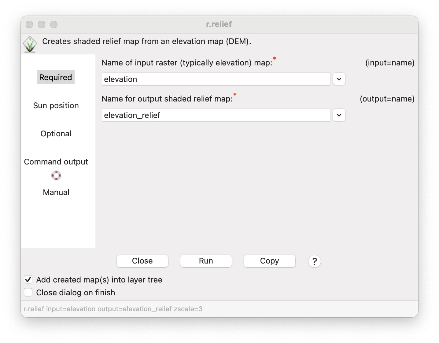
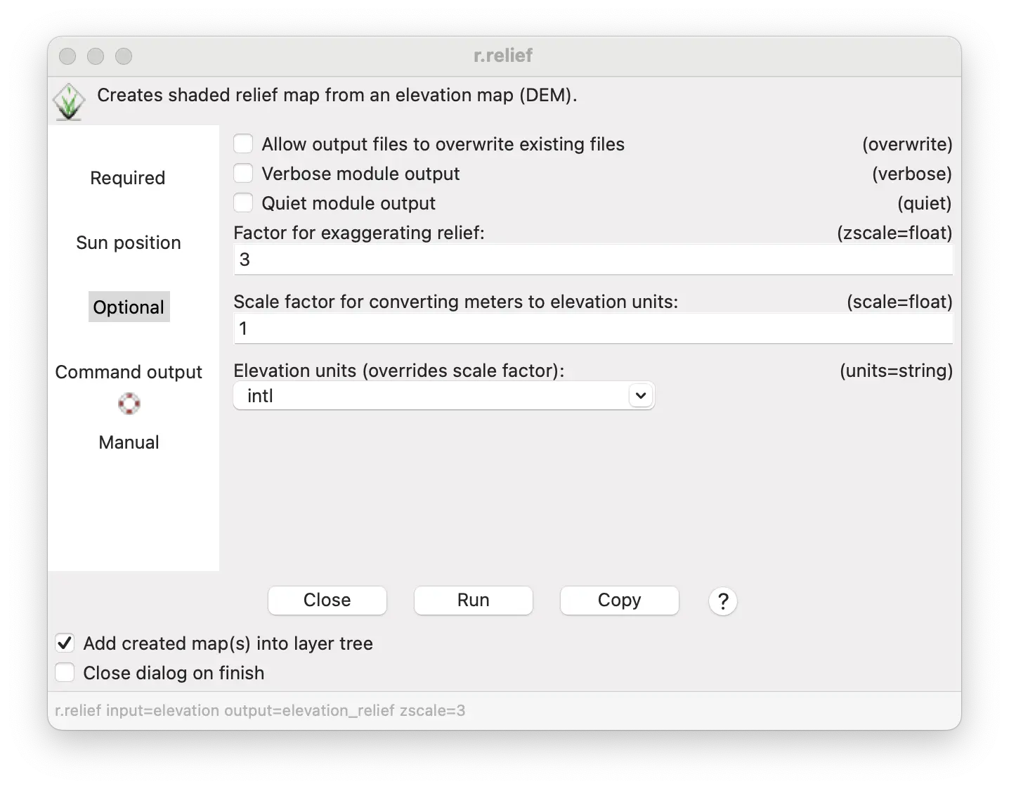
r.relief input=elevation output=elevation_relief zscale=3

Python

gs.run_command("r.relief", 
                input="elevation", 
                output="elevation_relief", 
                zscale=3)

Generating an RGB color map from image fusion

Use the r.composite tool from the Raster/Manage colors/Create RGB menu to create a new RGB map from the fusion of 3 PCA component maps.

GUI

1. Open r.composite

2. Enter the PCA component maps 1-3 into the red, green, and blue text entry boxes.

3. Enter Flagstaff_landsat8PCA_123_RGB as the output RGB map.

4. Press Run

Command line

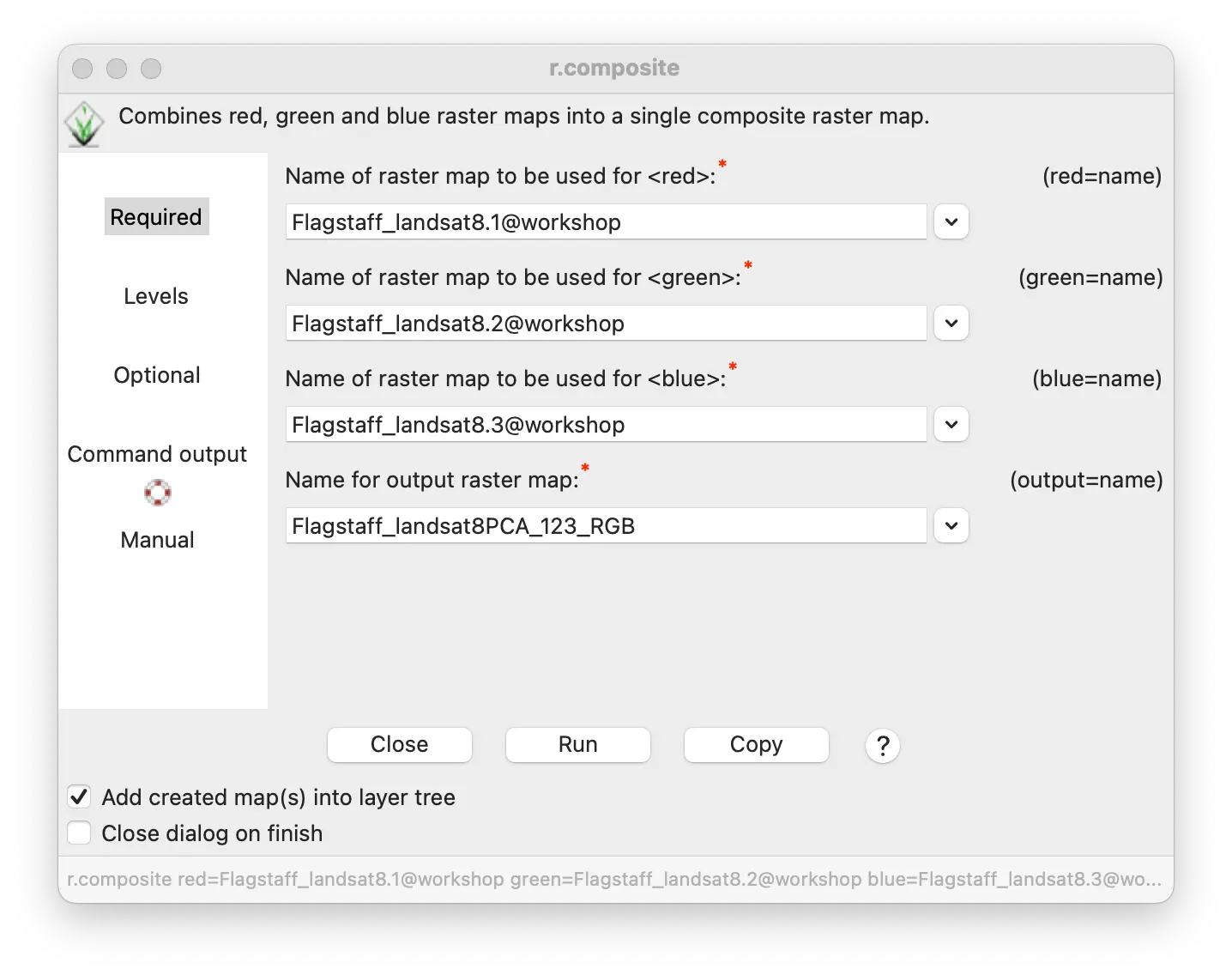
r.composite red=Flagstaff_landsat8.1 green=Flagstaff_landsat8.2 blue=Flagstaff_landsat8.3 output=Flagstaff_landsat8PCA_123_RGB

Python

gs.run_command("r.composite", 
                red="Flagstaff_landsat8.1", 
                green="Flagstaff_landsat8.2", 
                blue="Flagstaff_landsat8.3", 
                output="Flagstaff_landsat8PCA_123_RGB")

Combining relief and a color image fusion map

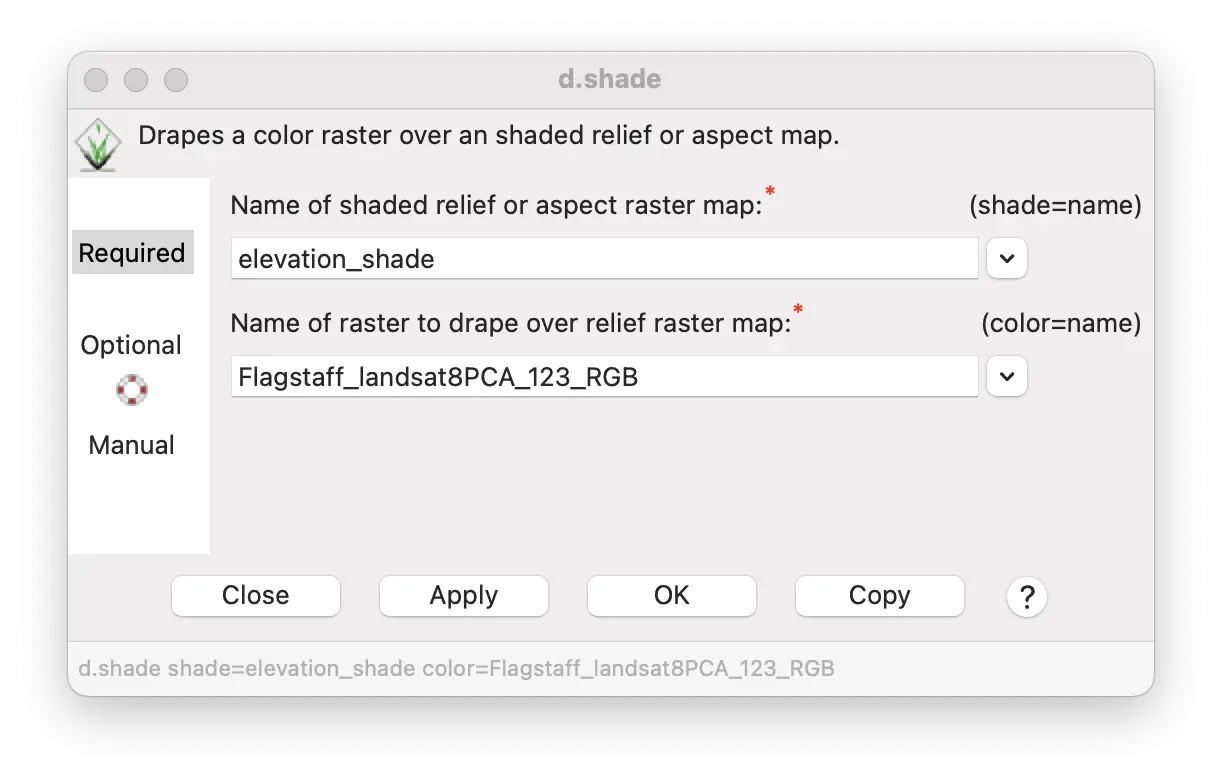
A topographic relief map and an RGB image fusion map can be combined with the d.shade tool in the layer manager or by using the r.shade tool from the /Raster/Terrain analysis/Apply shade to raster menu.

GUI

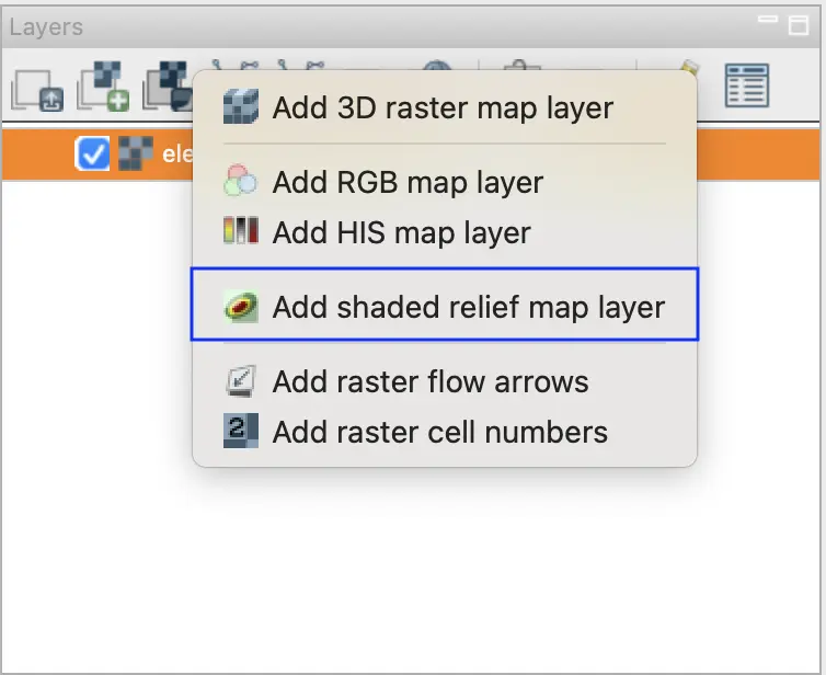
1. In the layer manager, select Add shaded relief map layer (d.shade tool) from the Add various raster map layers menu button.

2. Enter the elevation_relief map into the Name of shaded relief text box

3. Enter Flagstaff_landsat8PCA_123_RGB into the Name of raster to drape over relief text box.

4. If you set the Percent to brighten to 30 or 40, it will create a more visually appealing display.

5. To create a color shaded relief map, use the r.shade tool with the same entries as above for the Layer Manager and provide a name for the output map to be created (e.g., PCA_relief).

Command line

r.shade shade=elevation_relief color=Flagstaff_landsat8PCA_123_RGB output=PCA_relief  brighten=40

Python

gs.run_command("r.shade", 
                shade="elevation_relief", 
                color="Flagstaff_landsat8PCA_123_RGB", 
                output="PCA_relief", 
                brighten=40)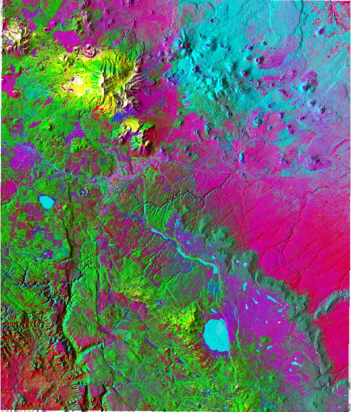

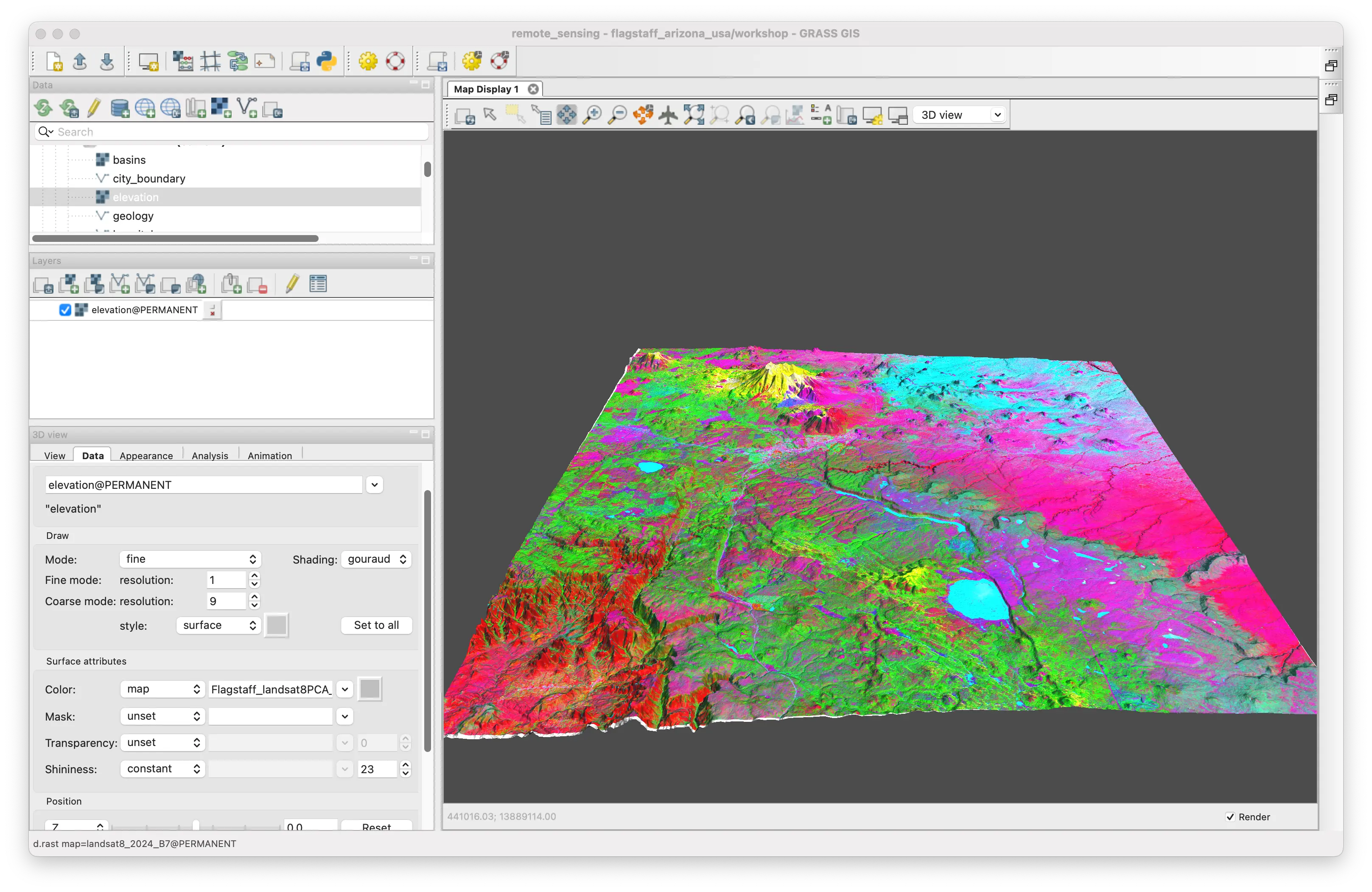
Relief map of topography shaded by RGB fusion of PCA components 1-3

Visualizing image fusion and topography in NVIZ

Additionally, the PCA image fusion can be used to color a 3D visualization of topography in GRASS’s 3D view using the NVIZ module.

• Start by opening the elevation DEM in the layer manager. Make sure that no other maps except elevation are displayed.
• Select 3D view from the pull-down menu at the top of the map display window. This should display the elevation map in 3D with the same shading seen in the 2D display.

DEM topography displayed in 3D

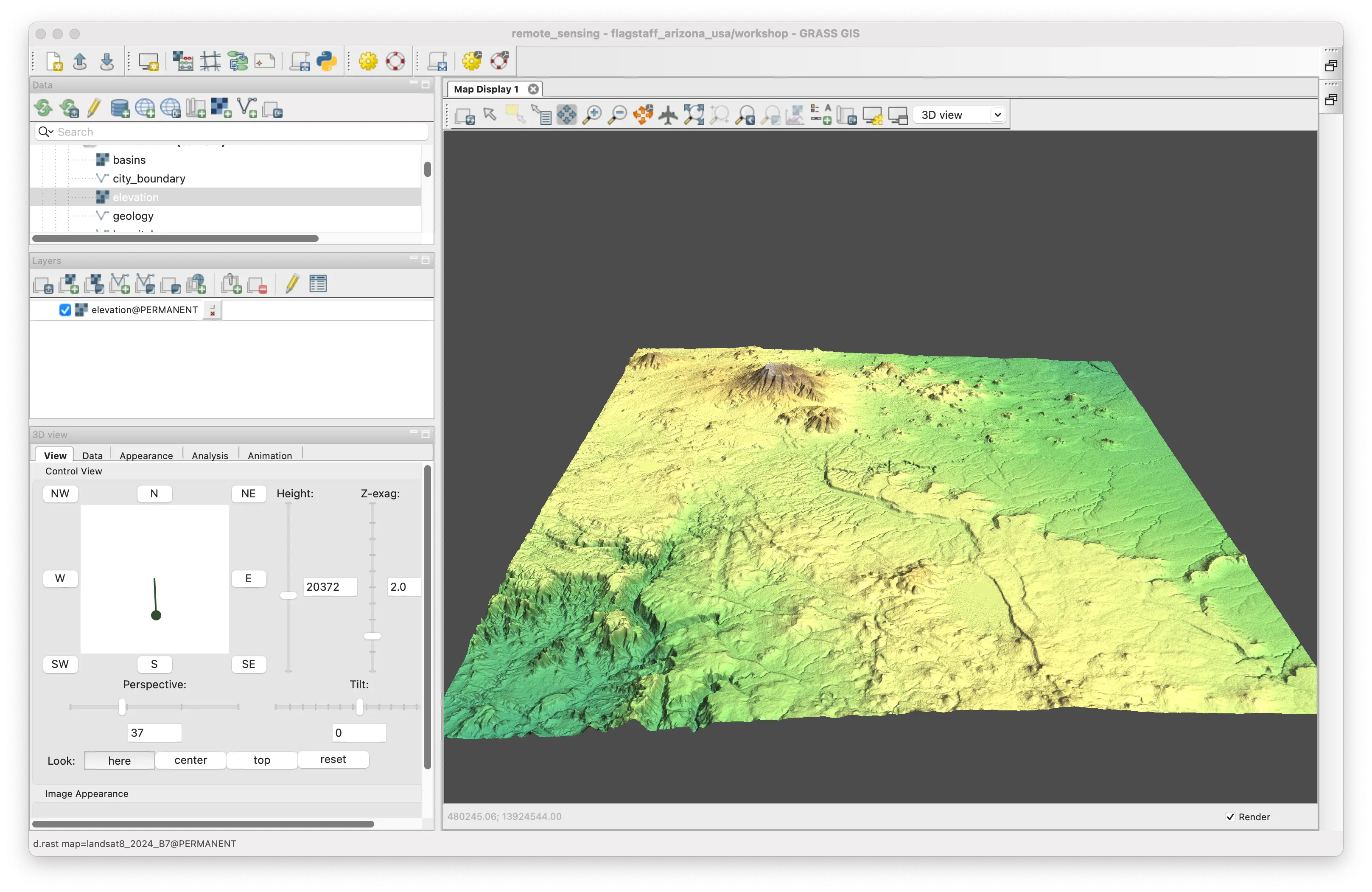
• Next, select the data tab in the 3D display manager window (It might be easier to manage the 3D display if you ‘tear’ it off from the side bar into a separate window). Make sure the elevation map is selected in the Raster map box at the top of the data window.

• Scroll down a bit to the Color section and replace the elevation map with the RGB raster map of the PCA 1-3 image fusion (Flagstaff_landsat8PCA_123_RGB).

DEM topography colored by PCA components 1-3 displayed in 3D

Advanced remote sensing with GRASS

GRASS has many more features and tools for working with remote sensing data.

• For satellite imagery, there are tools under the Imagery menu and in GRASS addons for

  • Image correction and calibration

  • Image georectification)

  • Machine learning algorithms for unsurpervised and supervised image classification and feature detection

  • Statistical analysis and visualization as demonstrated in this tutorial.

• Satellite time series can be transformed into time cubes for analysis with GRASS’s unique Temporal GIS tools.

• For aerial photography, there are tools for

  • Georectification

  • 3D rectification and scanning distortion for correction for orthophotography

  • Image enhancement, including neighborhood, convolving, edge detection, and fast fourier transform filters.

• GRASS has an extensive suite of raster and vector tools for processing and visualizing LiDAR data, as well raster and vector import and processing of LiDAR data.

• There are multiple methods for interpolation of data points from geophysical surveys.

• For 3D geophysics (e.g., electrical tomography or ground penetrating radar), GRASS offers a unique suite of true 3D voxel analysis tools with n-dimensional visualization in NVIZ.

These and other tools make GRASS a rich and powerful geoprocessing environment for many remote sensing applications.