g.region raster=elevation
r.mapcalc "friction0 = 0"Modeling Movement in GRASS
intermediate
advanced
GUI
raster
cost surface
least cost path
Generating a cumulative cost surface and least cost path with r.walk and r.path to model movement by walking across a landscape.
GRASS has sophisticated tools to model movement across terrain, including r.cost, r.walk, r.drain, and r.path. In this tutorial, we will use r.walk and r.path to determine the best walking path to reach a destination, like a hospital.
NoteDataset
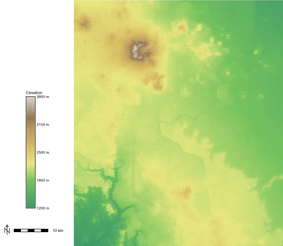
This tutorial uses one of the standard GRASS sample data sets: flagstaff_arizona_usa. We will refer to place names in that data set, but it can be completed with any of the standard sample data sets for any region–for example, the North Carolina data set. We will use the Flagstaff elevation DEM, the hospitals vector points file (any other vector point file will serve), and the landuse raster map.
This tutorial is designed so that you can complete it using the GRASS GUI, GRASS commands from the console or terminal, or using GRASS commands in a Jupyter Notebook environment.
NoteDon’t know how to get started?
If you are not sure how to get started with GRASS using its graphical user interface or using Python, checkout the tutorials Get started with GRASS GUI and Get started with GRASS & Python in Jupyter Notebooks.
What is a cost surface?
A cost surface is a raster in which each cell represents the “cost” or difficulty to move across landscape.
A cumulative cost surface shows the total accumulated cost of moving from a starting point to a location. Cumulative cost surfaces are also used to find a least cost path between a location and the starting point.
GRASS r.walk tool generates a cumulative cost surface using Naismith’s rule for walking times where each cell has the value in seconds of the time it takes to walk from the start point to that cell.
Modeling movement with a cumulative cost surface
Overview
Start with a DEM of elevation for topography to determine movement costs.
Create a friction map with a value of 0 (or other values for additional movement costs).
Select start point(s).
Create a cost surface.
A least cost path can then be calculated between any point on the cost surface and the start point.
Friction map
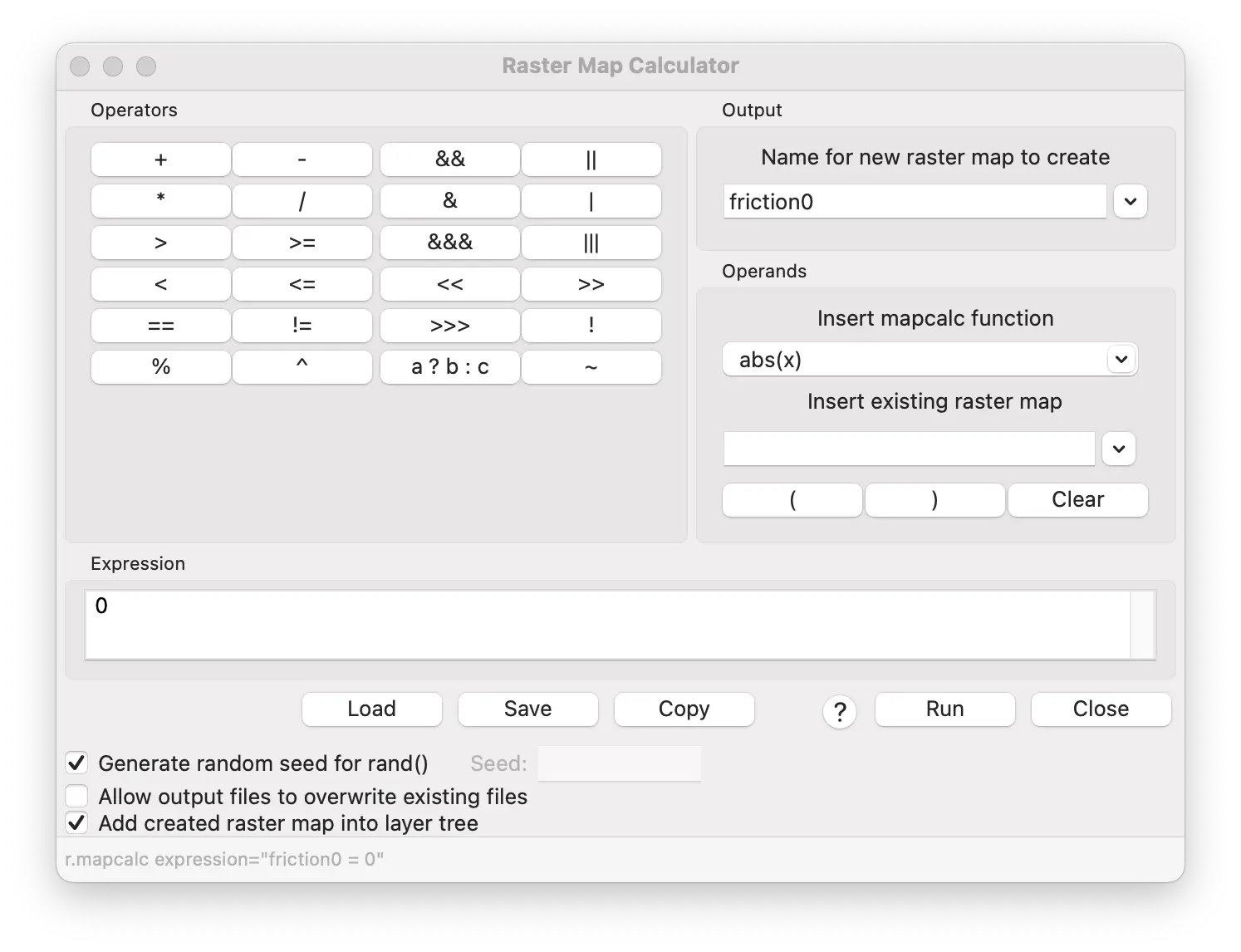
The GRASS map calculator lets you create a map, alter a map, or combine maps using map algebra. The map calculator can be used from the GUI or as a command.
Before you make a friction map, make sure the computational region matches the elevation map.
Create the friction0 map with 0 in every cell.
Add the elevation raster to the Layer Manager.
Right click elevation in Layer Manager.
Select Set computational region from selected map.
Open the Raster Map Calculator from the top toolbar (“abacus” icon).
Fill in the output map name as friction0 and enter 0 in the expression field.
Press Run.
Set the region to match the elevation map.
Create a friction map with a value of 0 in all cells that matches the extent and resolution of the elevation map.
Set the region to match the elevation map.
Create a friction map with a value of 0 in all cells that matches the extent and resolution of the elevation map.
gs.run_command("g.region", raster="elevation")
gs.mapcalc("friction0 = 0")Choose a start point
Now that we have a DEM map for terrain and a friction map, all we need for a cumulative cost surface is a start point: the point from which to calculate movement costs.
A start point can be a vector point, a raster cell, or even a pair of coordinates.
A cost surface in r.walk can have multiple start points.
We’ll make a start point from the Flagstaff Medical Center, found in the hospitals vector points file.
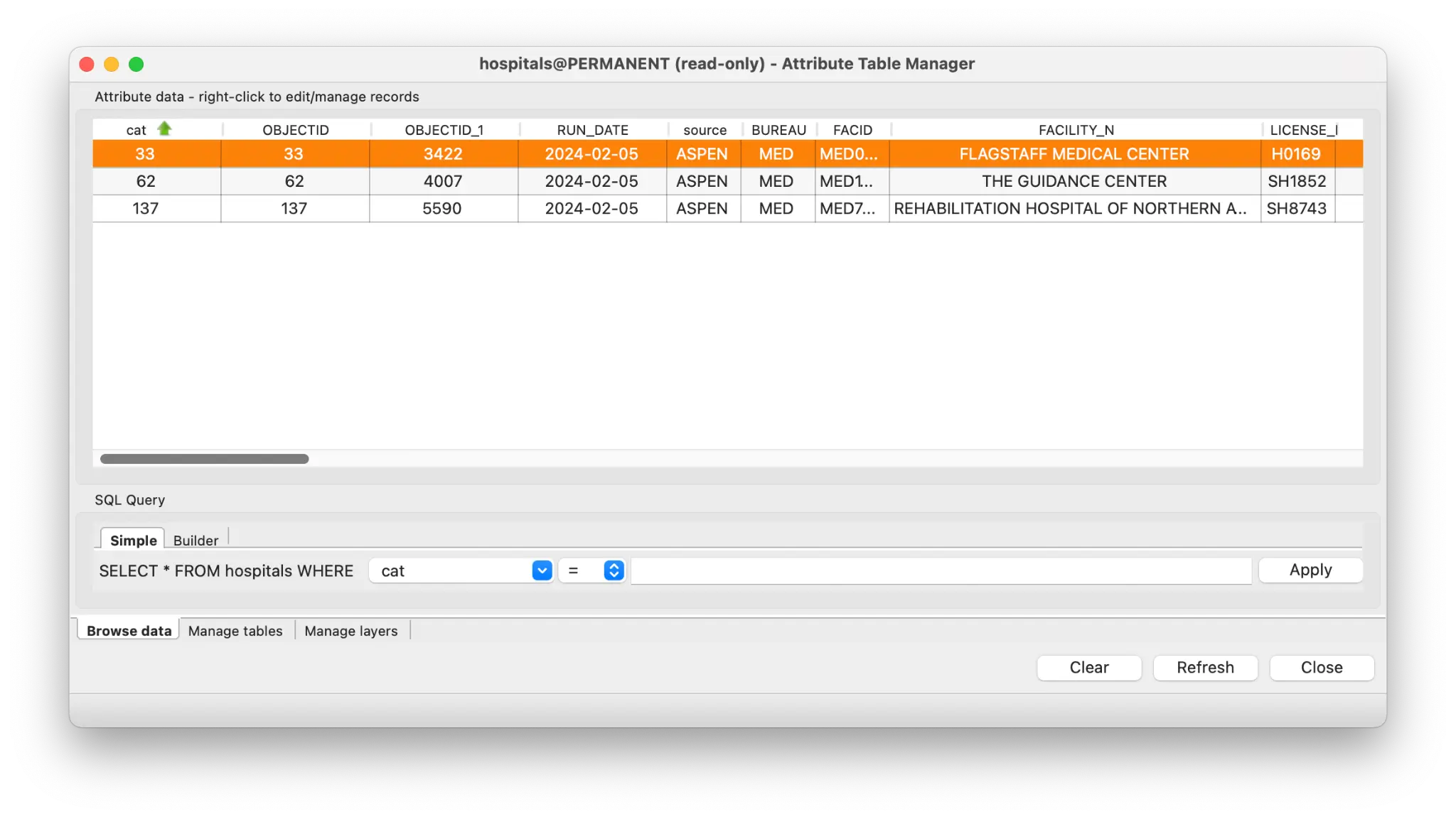
Use the Attribute Table Manager for hospitals:
Display hospitals map by adding it to the Layer Manager from Data Catalog.
Right click and open the Attribute Table Manager.
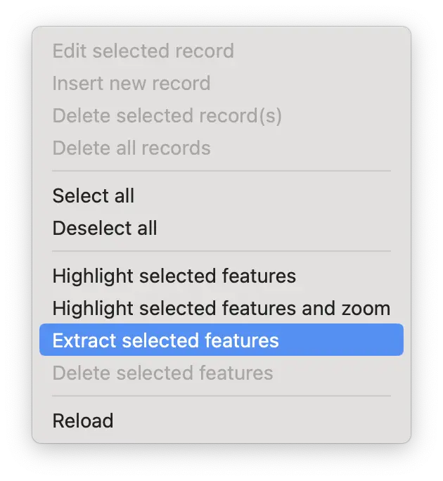
Select “Flagstaff Medical Center” record.
Right click and select Extract selected features from the context menu.
Name the new map FMC.
Use the v.extract tool to create a vector point map named FMC from the hospitals map.
v.extract input=hospitals type=point where="FACILITY_N = 'FLAGSTAFF MEDICAL CENTER'" output=FMCUse the v.extract tool to create a vector point map named FMC from the hospitals map.
gs.run_command("v.extract",
input="hospitals",
type="point",
where="FACILITY_N = 'FLAGSTAFF MEDICAL CENTER'",
output="FMC")- Use the d.vect tool by double clicking FMC in the layer manager to display the point with a color and size to see it better
Generate the cumulative cost surface
Use the r.walk tool from the Raster/Terrain Analysis menu.
- Enter the elevation map ( elevation ), friction map ( friction0 ), and name of the cost surface to create (FMC_cost_seconds).
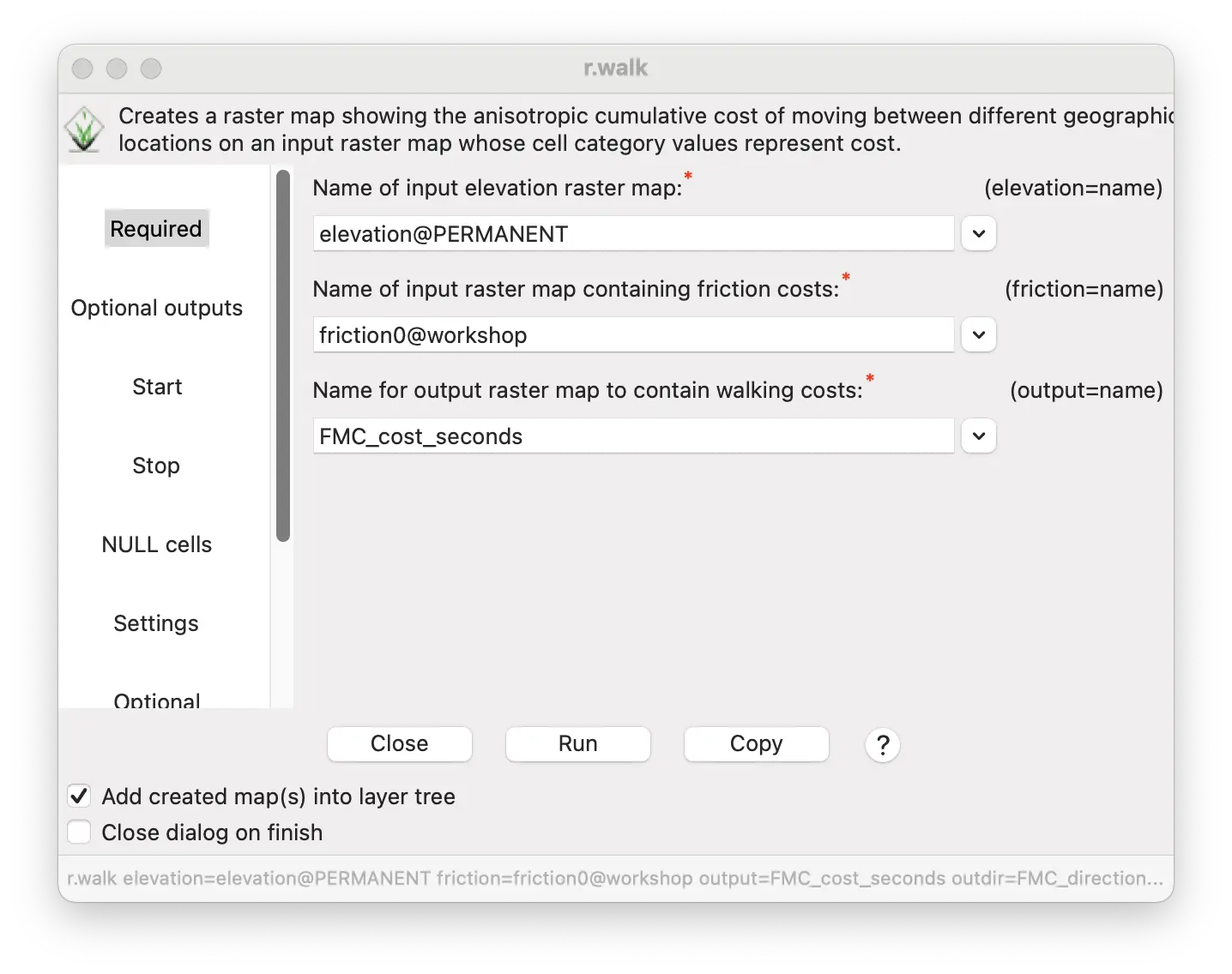
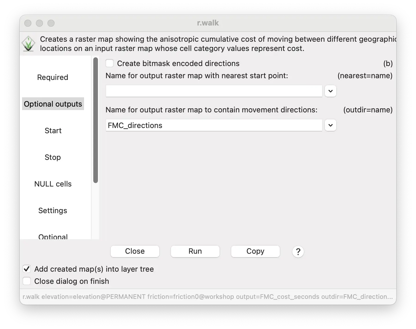
- Enter the name of a directions map ( FMC_directions ) to use for creating a least cost path.
- Enter the start point ( FMC ).
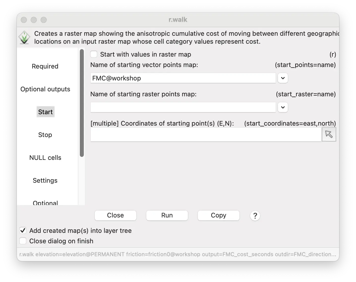
- Optional: control the spatial extent of cost surface.
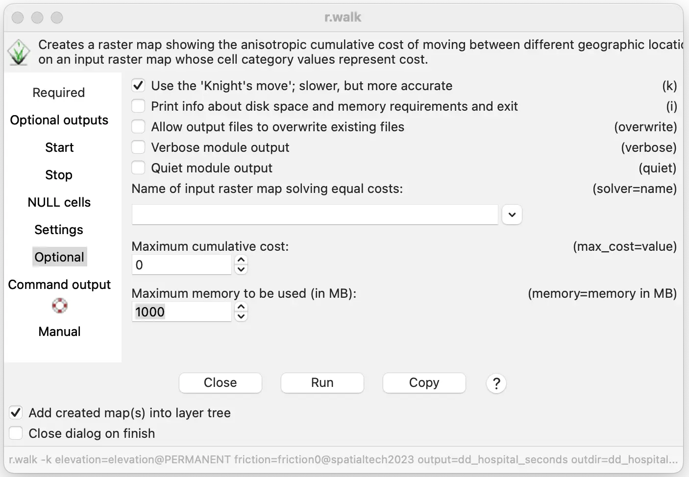
- Optional: adjust Movement parameter settings.

- Recommended: select knight’s move for calculating cost and direction.
NoteTip
Click the “copy” button to copy the GRASS command. You can save it in a text file for later reuse or to document your work.
- Use the r.walk command to generate the cumulative cost surface.
r.walk elevation=elevation friction=friction0 output=FMC_cost_seconds outdir=FMC_directions start_points=FMC -k- Use the r.walk command to generate the cumulative cost surface.
gs.run_command("r.walk",
elevation="elevation",
friction="friction0",
output="FMC_cost_seconds",
outdir="FMC_directions",
start_points="FMC",
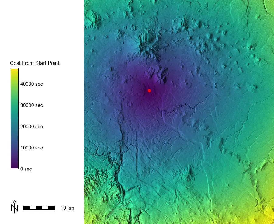
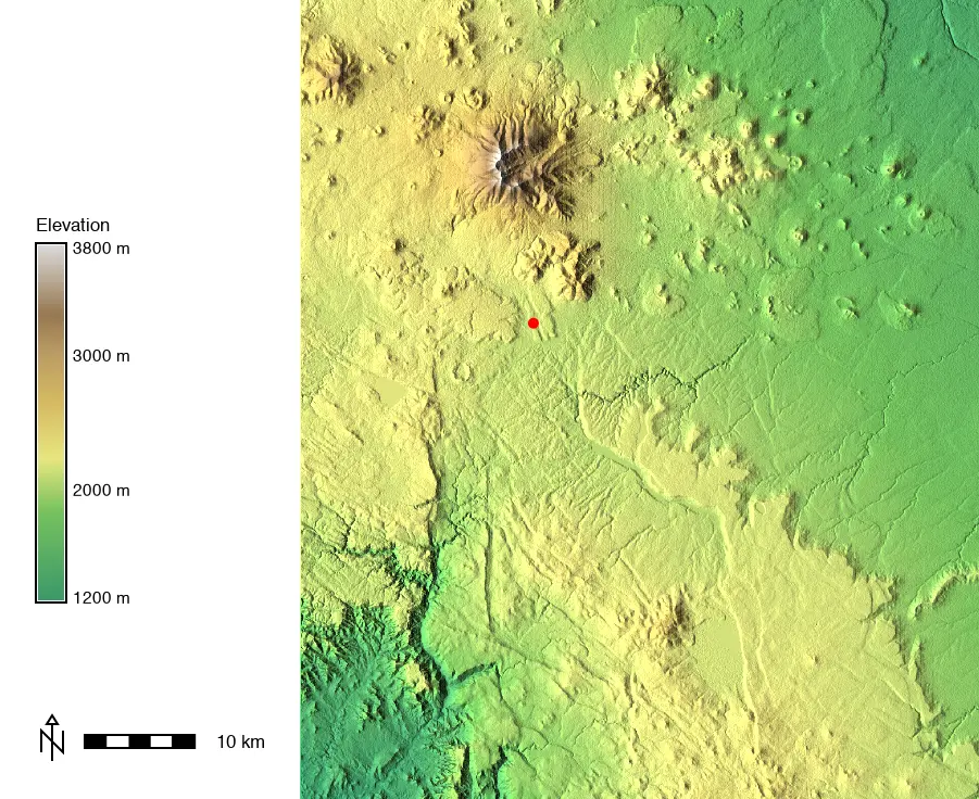
flags="k")Cumulative cost surface map
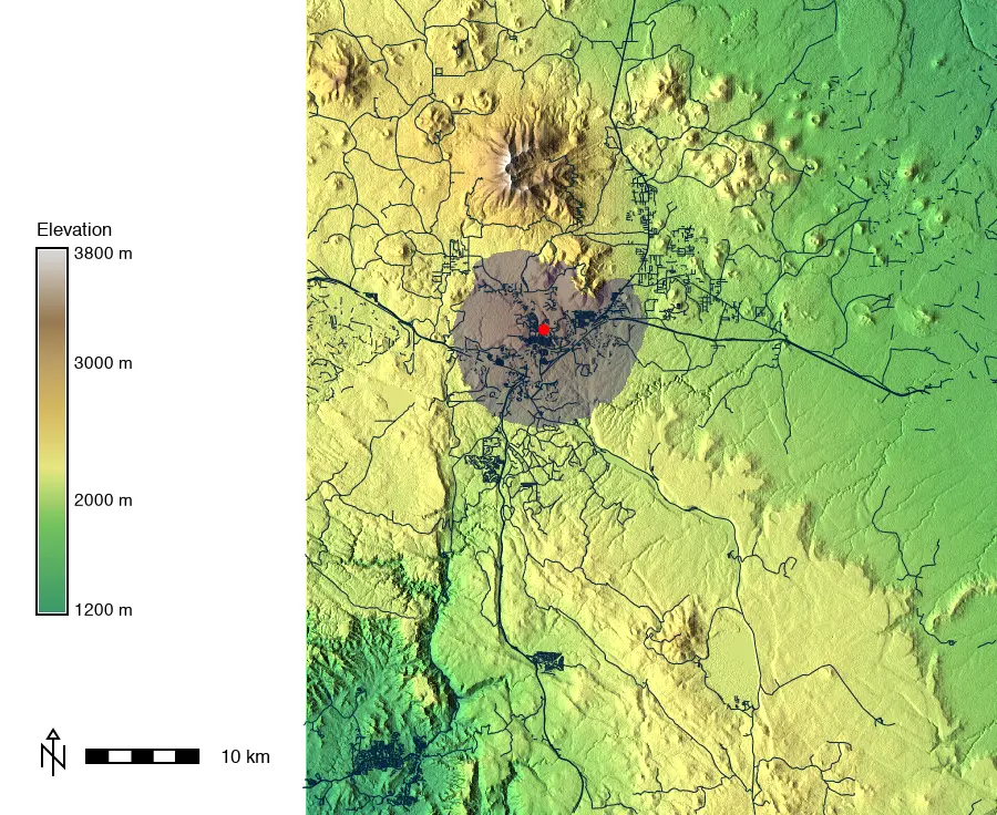
Each raster cell value in the cost surface is the time in seconds to walk from FMC to that cell over the terrain of the Flagstaff DEM.

Movement across a cumulative cost surface
You can transform the walking time in seconds to hours by dividing the map by 3600 using the map calculator.
Open the map calculator.
Enter the name of the new map of walking time in hours: FMC_cost_hours.
Enter FMC_cost_seconds / 3600 into the expressions field.
Press Run.
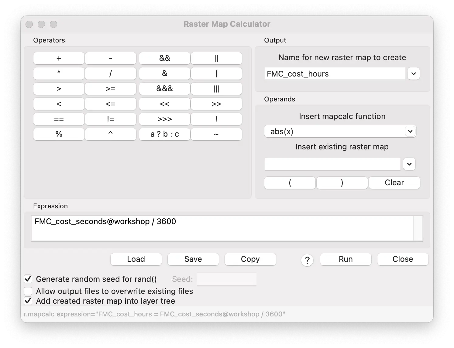
r.mapcalc "FMC_cost_hours = FMC_cost_seconds / 3600"gs.mapcalc("FMC_cost_hours = FMC_cost_seconds / 3600")We can query or filter this hourly cumulative cost surface to areas of equivalent walking time.
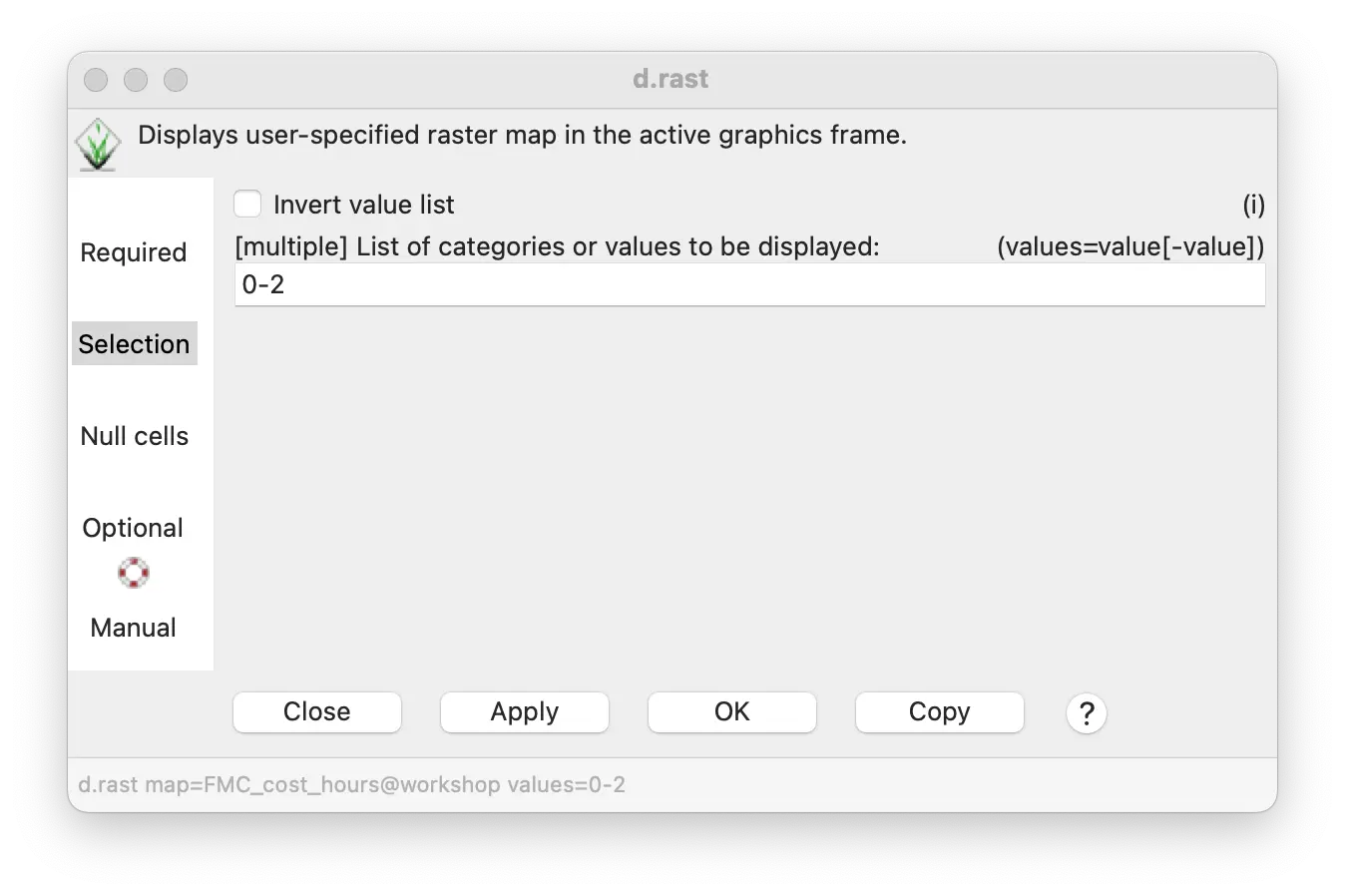
For example, in the layer manager we can used the d.rast tool to show the area within a 2 hour walk of FMC and then set the opacity of the cost surface to 50% to see the underlying terrain.
Least cost paths
Overview
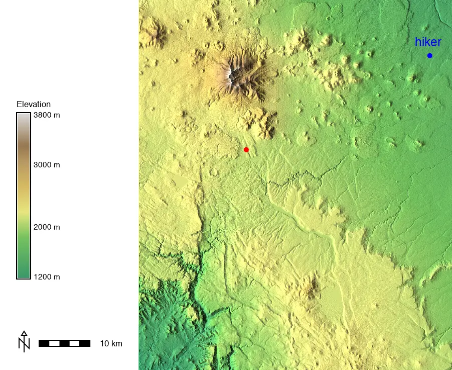
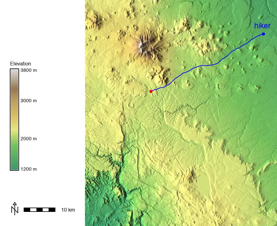
We can also plot a least cost path (LCP), which is the least costly (shortest time) route between any point on the cumulative cost surface and FMC.
Imagine a stranded hiker NE of Flagstaff who has to walk to FMC.
What path would take the least time?
Generating a least cost path
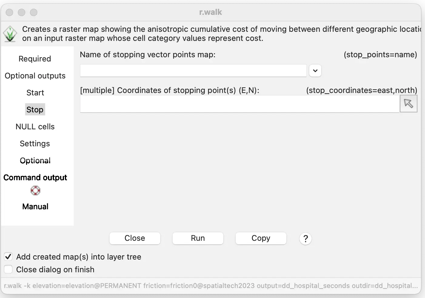
To create a LCP in GRASS, we will use r.path (also under the Raster/Terrain analysis menu).
- Input the directions map (FMC_directions) we also made when we created the cumulative cost surface.
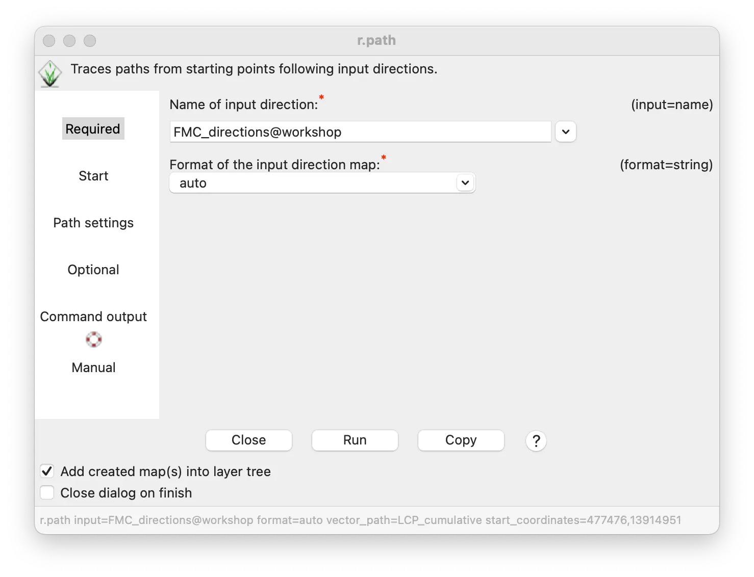
- Input the coordinates of the hiker (477476,3914951) as the starting point for the LCP. (We could also use a pre-defined vector point).
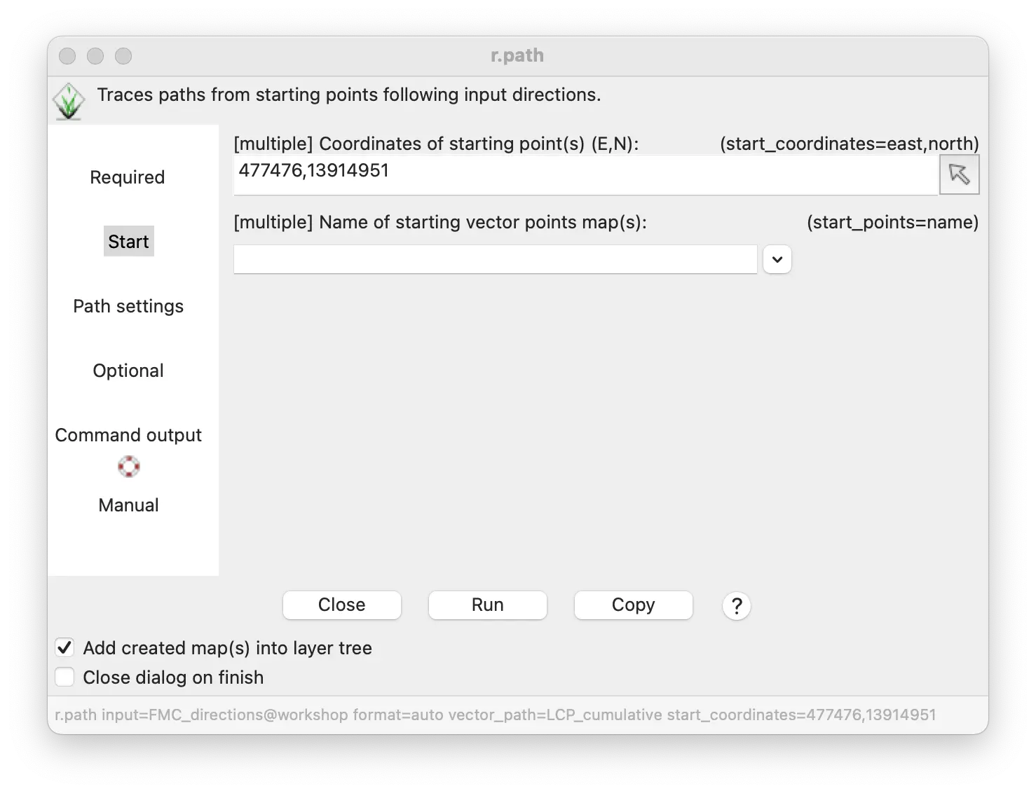
- Specify the name of the output vector path map (LCP_cumulative).
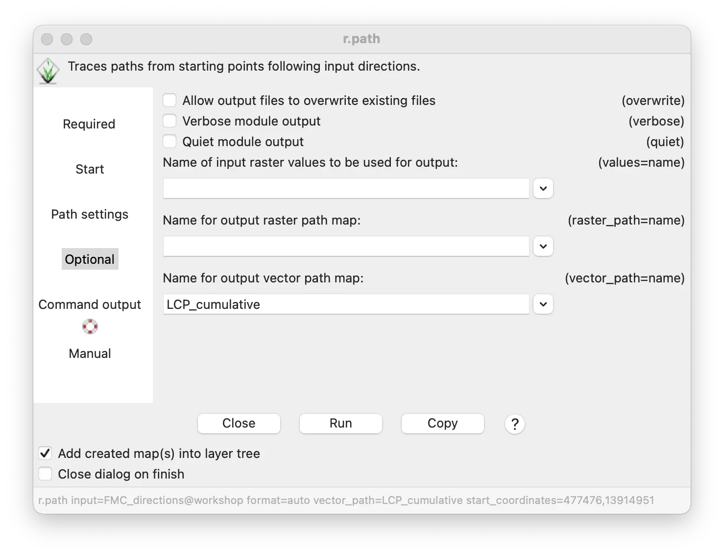
r.path input=FMC_directions format=auto vector_path=LCP_cumulative start_coordinates=477476,3914951gs.run_command("r.path",
input="FMC_directions",
format="auto",
vector_path="LCP_cumulative",
start_coordinates=[477476, 3914951])Least cost path generated
Here is the LCP result.
Adding a friction map to movement costs
Overview
A friction map can be used to incorporate other factors than just terrain into creating a cumulative cost surface and modeling movement.
The value of each cell in a friction map raster is the amount of walking time, in seconds/meter, in addition to the time needed because of terrain.
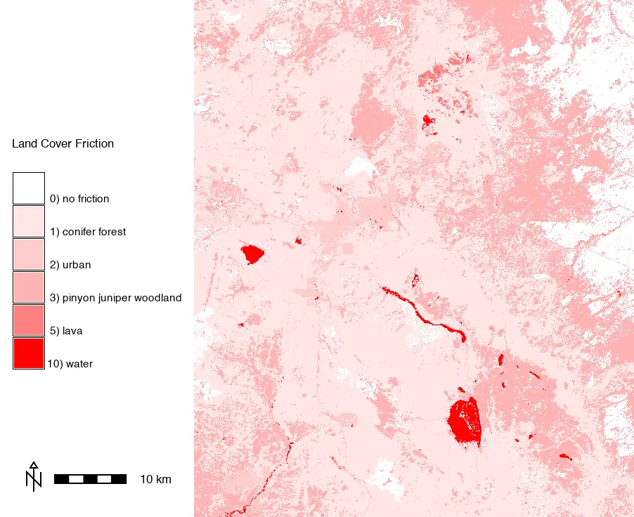
We can reclassify the landuse map to create a friction map of the amount of extra time it would take to walk through different kinds of land cover.
Reclassifying landuse to create a friction map
A standard walking speed across flat terrain is about 5 km/hr = 0.72 sec/m.
We might then estimate that it would take an additional
3 sec/m to walk through dense pinyon-juniper woodland
1 sec/m to cross conifer forest
2 sec/m to wander through urban Flagstaff
5 sec/m to clamber over lava fields
10 sec/m to try and cross water
We can create this friction map by reclassifying the landuse map using r.reclass to assign new friction values to the existing land cover categories.
The r.reclass tool is found under the Raster/Change category menu.
Enter landuse for the raster to be reclassified.
Enter friction_reclassified for the output reclassified map.
Enter the reclass rules directly in the text box or from a saved text file. Use and * symbol to represent everything not covered by the specific reclass rules.
11 90 95 = 10 water
21 thru 24 = 2 urban
31 = 5 lava
41 thru 43 = 1 conifer forest
52 = 3 pinyon juniper woodland
* = 0 no friction
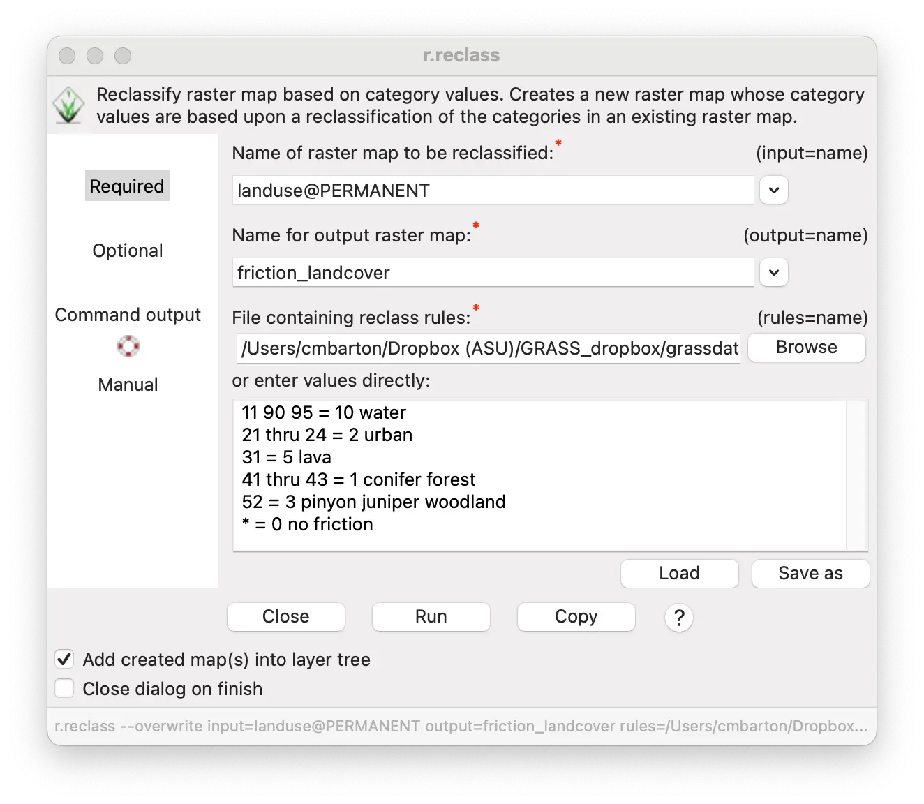
r.reclass input=landuse output=friction_landcover rules=- << EOF
11 90 95 = 10 water
21 thru 24 = 2 urban
31 = 5 lava
41 thru 43 = 1 conifer forest
52 = 3 pinyon juniper woodland
* = 0 no friction
EOFrules = """\
11 90 95 = 10 water
21 thru 24 = 2 urban
31 = 5 lava
41 thru 43 = 1 conifer forest
52 = 3 pinyon juniper woodland
* = 0 no friction
"""
gs.write_command("r.reclass",
input="landuse",
output="friction_landcover",
rules="-",
stdin=rules)This creates a new friction map named friction_landcover.
Modifying a cumulative cost surface with a friction map
We can now create a new cumulative cost surface using this new friction map and convert it from seconds to hours, as we did before.
Follow the procedures in the Generate the cumulative cost surface section and substitute the new friction_landcover map for the friction0 map used previously.
Convert the cumulative cost surface to hours instead of seconds following the procedures in the Movement across a cumulative cost surface section.
r.walk elevation=elevation friction=friction_landcover output=FMC_vegcost_seconds outdir=FMC_vegcost_directions start_points=FMC -k
r.mapcalc "FMC_vegcost_hours = FMC_vegcost_seconds / 3600"gs.run_command("r.walk",
elevation="elevation",
friction="friction_landcover",
output="FMC_vegcost_seconds",
outdir="FMC_vegcost_directions",
start_points="FMC",
flags="k")
gs.mapcalc("FMC_vegcost_hours = FMC_vegcost_seconds / 3600")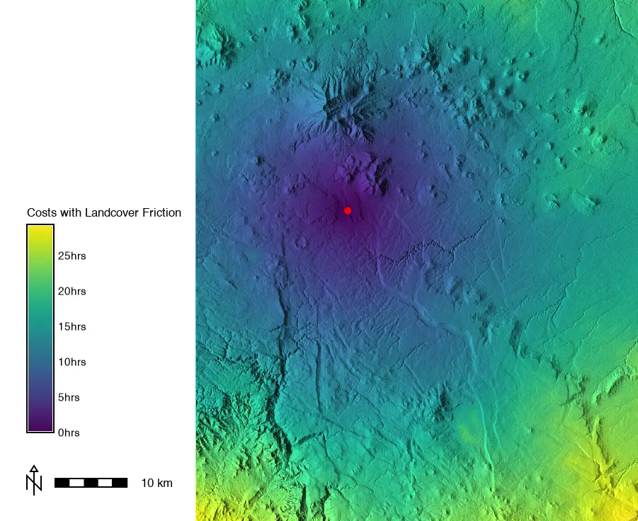
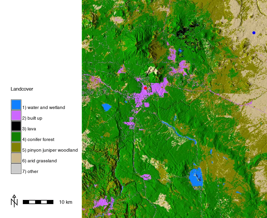
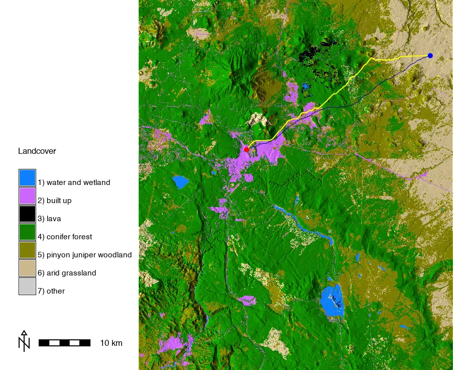
Least cost paths and friction
We can create a new LCP from the stranded hiker to FMC over terrain where land cover also affects the cost of movement.
Follow the procedures in the Least cost path section, substituting the new direction map made along with the cumulative cost surface with land cover friction map.
Give this new LCP the name LCP_vegcost to distinguish from the previous LCP.
r.path input=FMC_vegcost_directions format=auto vector_path=LCP_vegcost start_coordinates=477476,3914951gs.run_command("r.path",
input="FMC_vegcost_directions",
format="auto",
vector_path="LCP_vegcost",
start_coordinates=[477476, 3914951])It takes more time to reach FMC if the hiker has to navigate dense vegetation as well as terrain.
In the map below, terrain colored by land cover, the original LCP with terrain only is shown by the blue line. The LCP with a land cover friction map is shown by the heavier yellow line.
© Michael Barton and Anna Petrasova 2026 The development of this tutorial was funded in part by the US National Science Foundation (NSF), award 2303651.