grass -c EPSG:6543 /path/to/nc6543Hydro-flattening a Digital Elevation Model
Python
intermediate
topography
lidar
GUI
Learn how to do hydro-flattening of a DEM.
What is hydro-flattening?
Hydro-flattening is the process of modifying a digital elevation model (DEM) so that water surfaces—such as lakes, reservoirs, and wide rivers—appear flat and level, as they would on traditional topographic maps. This is essential for producing clean contour lines and realistic-looking terrain surfaces.
When DEMs are created from lidar data, water surfaces often appear irregular or noisy. This happens because lidar points alone don’t define sharp edges like shorelines, and without breaklines to guide surface generation, the triangulation step connects points across waterbodies in unrealistic ways. The result is a DEM with unnatural ripples or slopes on water surfaces, which not only looks incorrect but also leads to poor-quality contours and artifacts in derived products. Hydro-flattening addresses this by incorporating breaklines that enforce flat, level water surfaces and preserve topographic realism. Read more at USGS website.
In this tutorial, you’ll learn how to use GRASS to apply hydro-flattening techniques to lidar-derived DEMs using r.hydro.flatten addon following these steps:
- Create a mean ground raster data layer from lidar point cloud dataset.
- Install GRASS addons to extend functionality.
- Add an OGC Standard Web Map Service (WMS) to the GRASS Map Display
- Create flat elevation data and edge standard deviation data raster layers for all areas of ground point voids in the lidar point cloud.
- Create 2D vector break lines and river center lines using the GRASS vector editor.
- Create automatic river transects
- Create hydro-flattened river raster data for inclusion in a DEM
- Create a filled DEM layer combining the mean ground data, hydro-flattened data, and other interpolated data.
- Export the resulting data from a GRASS project to a GeoTIFF file.
Getting ready
To get ready for the analysis, we will need to download lidar data, orthoimagery and install the r.hydro.flatten addon.
NoteDon’t know how to start using GRASS?
If you are not sure how to download and get started with GRASS using its graphical user interface or using Python, checkout the tutorials Get started with GRASS GUI and Get started with GRASS & Python in Jupyter Notebooks.
To create a raster surface from LiDAR point cloud data, GRASS must be compiled with the PDAL libraries. This capability is currently only available on Linux and OSX platforms and will be available on Windows when GRASS switches to the cmake-based build system (in development). In the meantime, the mean ground raster surface needed for the hydroflattening portion of the tutorial can be created on Windows using the QGIS point cloud tools. Create a virtual point cloud and then export it to raster (selecting classes 2,10,13 and setting the output resolution to 3.2808 ft).
Download data
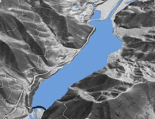
We will download lidar dataset from USGS website. Search for Lake Logan, North Carolina or use this bounding box:
-82.933790°, 35.423316°
-82.922031°, 35.407718°
Look for 2018 project lidar and download 6 lidar tiles as LAZ files. The coordinate reference system of the data is NAD83(2011) / North Carolina (ftUS) (EPSG:6543).
Now create a text file (laslist.txt) with a list of the 6 downloaded file and include the full path, for example:
/path/to/lidar/USGS_LPC_NC_Phase5_2018_A18_LA_37_00862212_.laz
/path/to/lidar/USGS_LPC_NC_Phase5_2018_A18_LA_37_00862320_.laz
/path/to/lidar/USGS_LPC_NC_Phase5_2018_A18_LA_37_00863205_.laz
/path/to/lidar/USGS_LPC_NC_Phase5_2018_A18_LA_37_00863209_.laz
/path/to/lidar/USGS_LPC_NC_Phase5_2018_A18_LA_37_00863317_.laz
/path/to/lidar/USGS_LPC_NC_Phase5_2018_A18_LA_37_00862208_.laz
We will use this file later on.
Start GRASS and create a new project
If this is the first time you have opened GRASS you will see the default startup screen with a WGS84 world project. Click on the Create new project button on the left or look for  on the upper left.
This will open a wizard where you:
- provide a name for the new project (e.g., nc6543), click Next
- specify Select CRS from a list by EPSG or description, click Next
- find EPSG 6543 and select it from the list, click Next
- select default datum transformation, click Next
- see summary and click Finish
gs.create_project("/path/to/nc6543", epsg="6543")Import data
The next step is to import the ground point data from the 6 lidar tiles to create a seamless mean ground elevation layer at 1m resolution. The data is in NC State Plane Feet, so we will be using a conversion factor of 3.28084 to convert the feet to meters for the resolution.
Fortunately, the GRASS tool r.in.pdal automates several aspects of this process.
Click on File → Import Raster Data → Point cloud (LAS LiDAR) import.
This will bring up the r.in.pdal dialog, that has multiple tabs that allow for several parameters for processing the point cloud data into a 2D raster.
- Input: for the file option browse to the laslist.txt.
- Output: check the boxes for Use the extent of the input for the raster extent, and Set computation region to match the new raster map. Type in
lake_logan_1mfor the Name for the output raster map. Type in 3.28084 for the Output raster resolution (the desired cell size is 1 meter). - Statistic: keep mean, this means that for the points that fall in each cell, the mean Z value will be calculated and set as the cell value.
- Selection: input 2,10,13 in the Only import points of selected classes field. Class 2 is ground, class 13 are roads and class 10 was used to designate ground points that were within 1 meter of 3D break lines for water bodies. These classes will get us the complete ground point dataset.
- Projection: check Reproject to project’s coordinate system if needed.
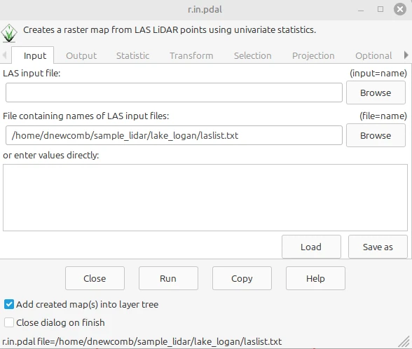
Now press run and wait. You should see the layer added to the map, if you don’t see it, right click on the layer and select Zoom to selected map(s). From the same context menu you can select Metadata to see number of cells, CRS information, extent, range of values and other info.
r.in.pdal -e -n -w file=/path/to/lidar/laslist.txt output=lake_logan_1m resolution=3.28084 class_filter=2,10,13
r.info map=lake_logan_1m
gs.run_command(
"r.in.pdal",
flags="enw",
file="/path/to/lidar/laslist.txt",
output="lake_logan_1m",
resolution=3.28084,
class_filter=[2, 10, 13],
)
print(gs.read_command("r.info", map="lake_logan_1m"))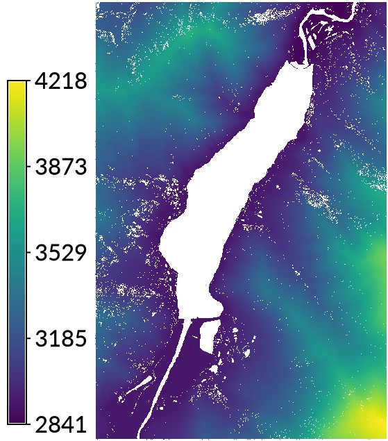
NoteOverwriting data
By default, GRASS prevents overwriting existing maps to protect your data, so you need to explicitly allow overwriting when re-running analyses or generating outputs with the same name. In a tool dialog, check Allow output files to overwrite existing files. In command line, use --o, and in Python, use overwrite=True.
Download orthoimagery
The State of North Carolina has a program to collect aerial imagery on a 4 year cycle. The most current data set for this location is from 2023. The URL to access the WMS data set is https://services.gis.nc.gov/secure/services/Imagery/Orthoimagery_2023/ImageServer/WMSServer.
Data is also available for 2019, 2015, and 2010, just substitute those years for 2023 in the URL above if you wish to review those years.
To display it, add web service layer:
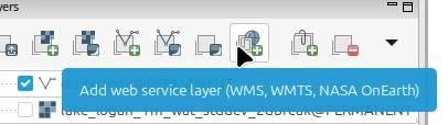
and paste the URL into the Server settings text box and press Connect. Select the newly populated layer Orthoimagery (2023). Select Source projection EPSG:6543 to match your project’s CRS for faster response. Also select the jpeg radio button in the Source image format.
To remember the URL, click on the Save button on the top of the dialog and enter a descriptive name to quickly recall the image service between sessions.
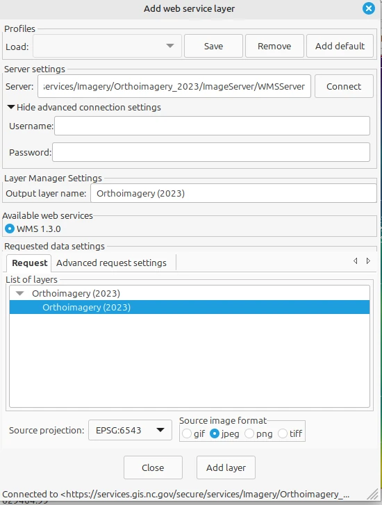
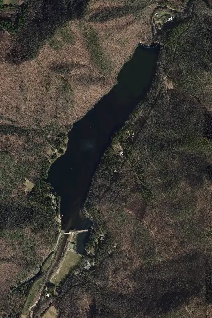
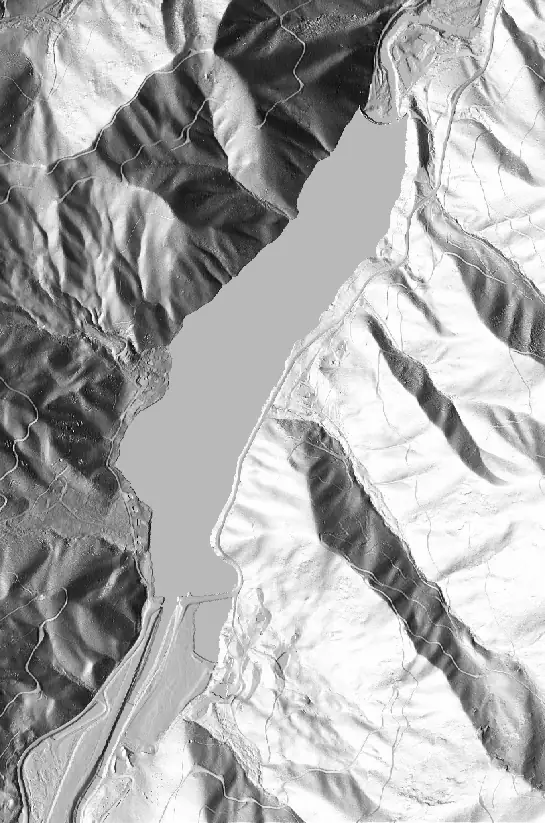
Click Add layer. Your GUI should now have Orthoimagery (2023) listed as one of the layers. Uncheck the orthoimagery layer and zoom into one of the void areas to the left of the lake. Once you have zoomed in, check the orthoimagery layer and see what the void represents.
r.in.wms layers=0 output=ortho srs=6543 url=https://services.gis.nc.gov/secure/services/Imagery/Orthoimagery_2023/ImageServer/WMSServergs.run_command(
"r.in.wms",
layers=0,
output="ortho",
srs="6543",
url="https://services.gis.nc.gov/secure/services/Imagery/Orthoimagery_2023/ImageServer/WMSServer",
)
Installing r.hydro.flatten addon
GRASS Addons are installed in the GUI with Addons extensions→ Install extensions from addons. In the dialog, search for the addon and Install.
At this point, you could run r.hydro.flatten from the command line, but it would be easier going forward if the command was integrated into the Tools tab. Restarting GRASS will automatically load the r.hydro.flatten tool in the Addons portion of the Tools tab. In the quit confirmation dialog click on Quit GRASS. The store curent settings dialog will then pop up, select No. Start GRASS again. You should now see an Addons option in the Tools tab with r.hydro.flatten listed there. Double click on r.hydro.flatten tool to open a dialog.
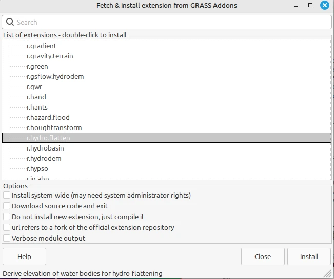
g.extension extension=r.hydro.flattengs.run_command("g.extension", extension="r.hydro.flatten")Hydro-flattening Lake Logan
Now we are ready to compute the hydro-flattened DEM. The r.hydro.flatten addon will calculate the estimated elevations of the voids from the 14th percentile of the edge values of each void in the ground point data and the standard deviation of the edge values around each void.
In the r.hydro.flatten dialog, set the following input and output values:
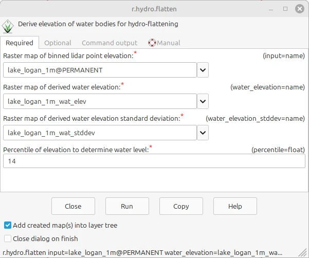
r.hydro.flatten input=lake_logan_1m water_elevation=lake_logan_1m_wat_elev water_elevation_stddev=lake_logan_1m_wat_stddev percentile=14gs.run_command(
"r.hydro.flatten",
input="lake_logan_1m",
water_elevation="lake_logan_1m_wat_elev",
water_elevation_stddev="lake_logan_1m_wat_stddev",
percentile=14,
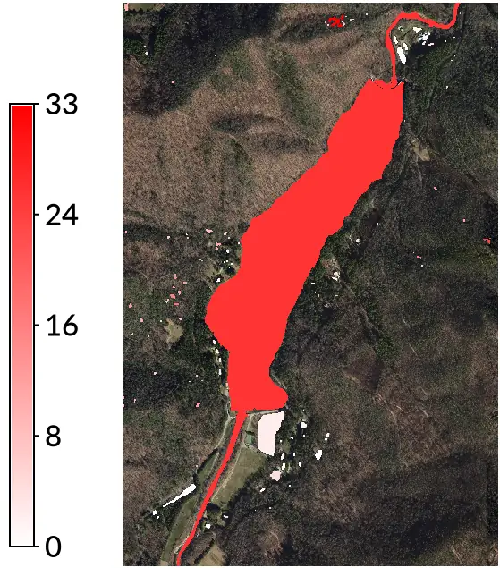
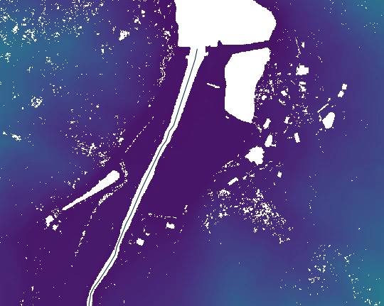
)Let’s inspect the newly created lake_logan_1m_wat_stddev raster that represents the standard deviation of elevation values along the edge of the water bodies. As you can see, the pond below the dam has such a low value that it is almost white. This means the hydro-flattening tool successfully flattened the pond surface.
However, the river upstream of the main lake (southwest), the lake, and the river downstream of the lake (northeast) all seem to have the same color. This happens because the elevation is calculated based on edge values, and the edges of the river and lake are treated as one continuous surface.
To improve accuracy, we need to interrupt that continuity by drawing 2D break lines in a vector layer—one where the river flows into the lake and another at the dam.
Since rivers are not perfectly level like lakes or ponds, we also need to add transects—short cross-sections—along the river. These help capture gradual changes in elevation along the flow direction and ensure a more realistic representation of the river surface.
Adding break lines
We will manually add a break line to separate the lake from the river on both sides.
Additionally, we will digitize a centerline representing the river and create transects in an automated way by using v.transects tool.
Creating centerlines
We will start a vector digitizer from the Map Display toolbar (combo box at the end of the toolbar).
When the digitizer toolbar appears, select New vector map and type a name for it, such as centerlines. Create it and then you can close the newly opened attribute manager dialog, we won’t need it.
Now start digitizing a centerline, it doesn’t have to be perfect. Select Digitize new line tool from the toolbar and start digitizing from the edge with right click. To end line, use left click. Do it for both segments of the river. Quit digitizer.
NoteAutomated centerlines
For longer river segments you can use v.centerline for automated centerline generation.
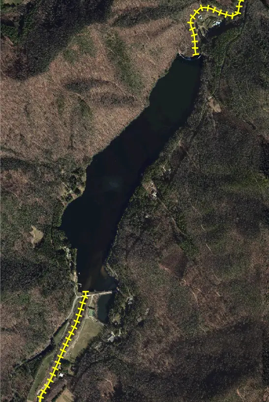
Creating river transects
Install v.transects addon in the same way as we installed the r.hydro.flatten one.
In the GUI dialog set the following values:
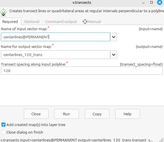
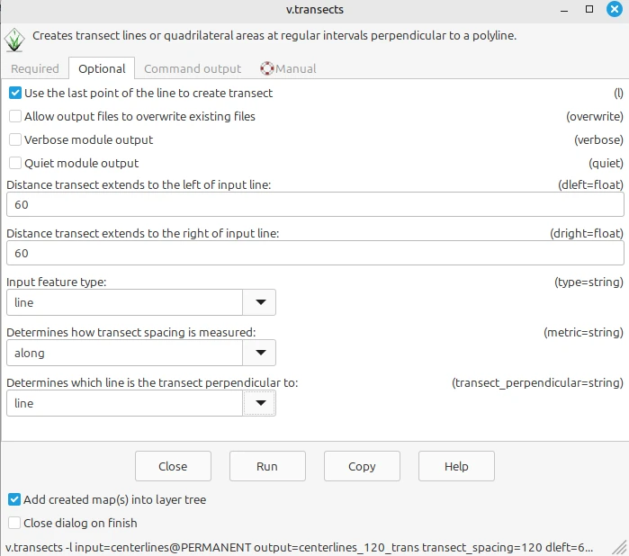
v.transects input=centerlines output=centerlines_120_trans transect_spacing=120 dleft=60 dright=60 metric=along transect_perpendicular=line -lgs.run_command(
"v.transects",
input="centerlines",
output="centerlines_120_trans",
transect_spacing=120,
dleft=60,
dright=60,
metric="along",
transect_perpendicular="line",
flags="l",
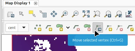
)Once the output transect layer is added to the Layers panel you will see the transects generated on the Map Display. You will note that some of the transect do not exactly line up with the shoreline correctly. Right click on the transect vector layer and select Start editing to bring up the vector editing toolbar. Select the Move selected vertex tool and use it to select and move the ends of the line to line up correctly. (Left click to select, left click to select new location, right click to complete move.)
Digitizing dam
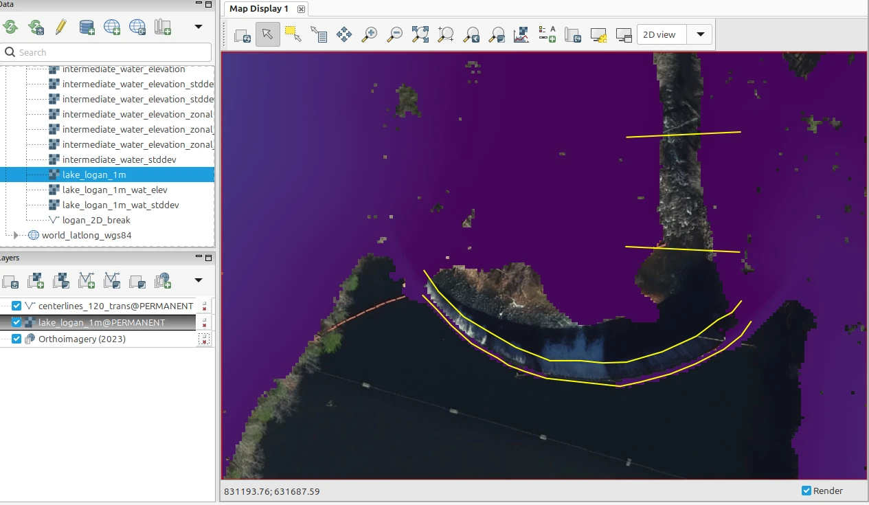
We will continue digitizing the centerlines_120_trans layer by adding breaklines on both sides of the dam.
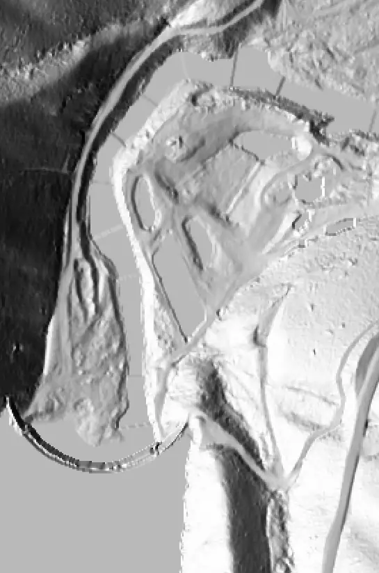
Zoom in to the north side of the lake where you see the semicircle of the dam, and click on the add line tool in the toolbar. In the orthophoto, you can see the dam line at the top of the dam. The first transect is placed at approximately the downstream edge of the plunge pool below the dam. It’s probably a good idea to put a break line at the base of the dam as well. Digitize the line along where you see the dam structure meet the water and save it.
Hydro-flattening with break lines
Let’s re-run r.hydro.flatten with the created break lines. This time, use centerlines_120_trans as your input vector layer and output resulting raster with filled DEM.
In the GUI dialog set the following values in the Optional tab. In the Required tab, add _2dbreak to the output names.
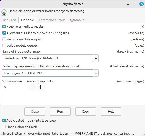
r.hydro.flatten input=lake_logan_1m water_elevation=lake_logan_1m_wat_elev_2dbreak water_elevation_stddev=lake_logan_1m_wat_stddev_2dbreak percentile=14 breaklines=centerlines_120_trans filled_elevation=lake_logan_1m_filled_DEMgs.run_command(
"r.hydro.flatten",
input="lake_logan_1m",
water_elevation="lake_logan_1m_wat_elev_2dbreak",
water_elevation_stddev="lake_logan_1m_wat_stddev_2dbreak",
percentile=14,
breaklines="centerlines_120_trans",
filled_elevation="lake_logan_1m_filled_DEM",
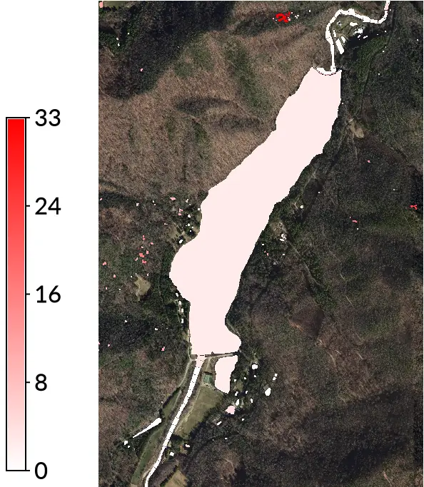
)Looking at the new standard deviation layer you will see that the lake and river are very light, indicating that the edge values for the lake and most of the river sections have relatively low standard deviation values.
There is a red spot in the top center of the study area. If you look at the area on the orthoimagery, you see dense evergreen vegetation. This is an area with a substantial void in the ground points that is not water. We don’t want this area to be flat, rather we will properly interpolate it.
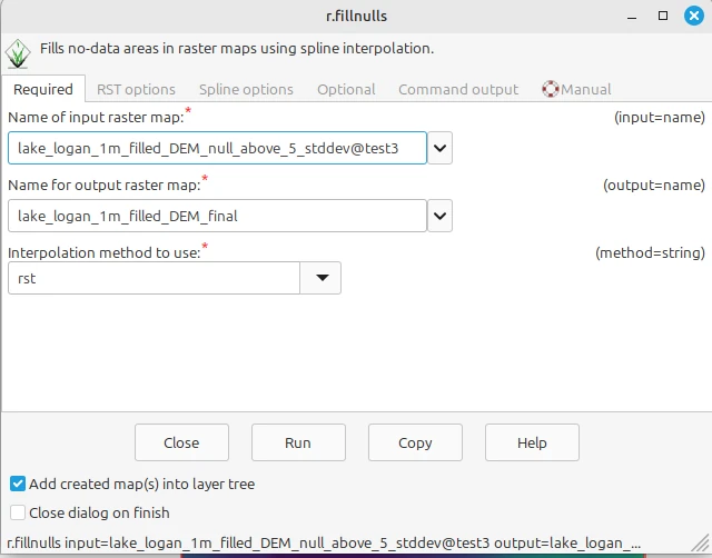
To avoid filling areas with standard deviation higher than a certain value, we will re-run r.hydro.flatten with parameter max_stddev and then fill those values with r.fillnulls.
Re-run the r.hydro.flatten with parameter max_stddev=5 to avoid flattening areas with standard deviation greater than 5. Name the resulting layer lake_logan_1m_filled_DEM_null_above_5_stddev.
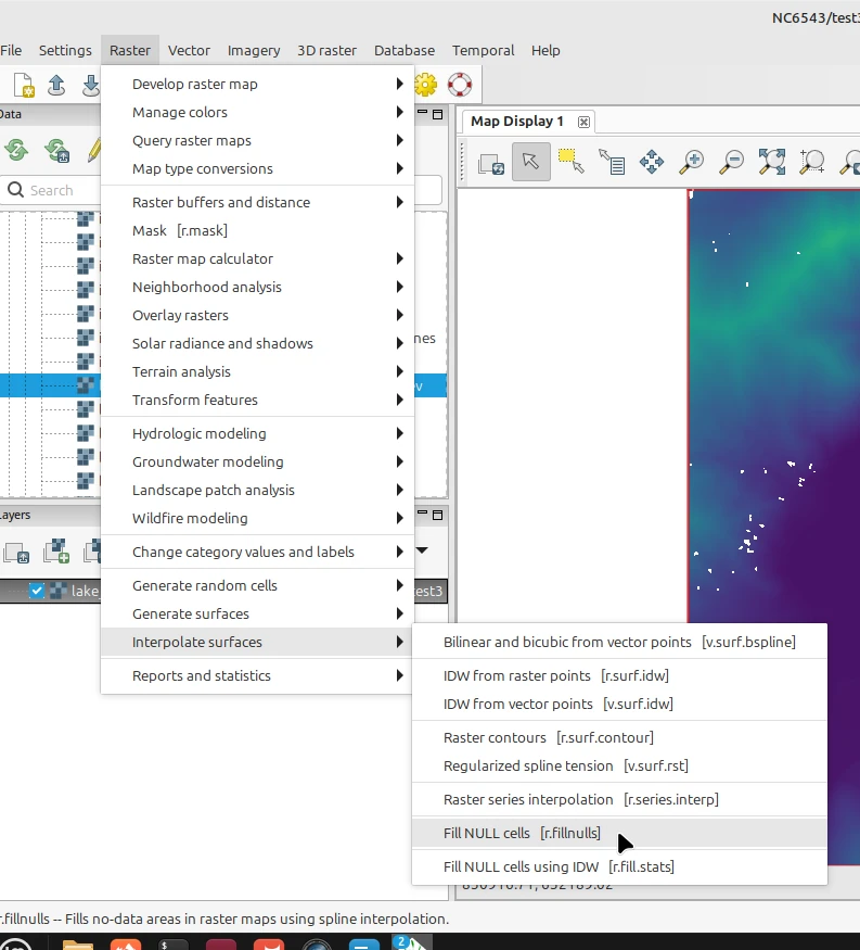
Then find r.fillnulls tool in menu Raster → Interpolate surfaces → Fill NULL cells and call r.fillnulls with input layer lake_logan_1m_filled_DEM, output layer lake_logan_1m_filled_DEM_fillnulls and keep the rest with the default values.
Finally, run r.relief to see the resulting topography.
r.hydro.flatten input=lake_logan_1m water_elevation=lake_logan_1m_wat_elev_2dbreak water_elevation_stddev=lake_logan_1m_wat_stddev_2dbreak percentile=14 breaklines=centerlines_120_trans filled_elevation=lake_logan_1m_filled_DEM_null_above_5_stddev max_stddev=5
r.fillnulls input=lake_logan_1m_filled_DEM_null_above_5_stddev output=lake_logan_1m_filled_DEM_final method=rst
r.relief input=lake_logan_1m_filled_DEM_final output=relief
gs.run_command(
"r.hydro.flatten",
input="lake_logan_1m",
water_elevation="lake_logan_1m_wat_elev_2dbreak",
water_elevation_stddev="lake_logan_1m_wat_stddev_2dbreak",
percentile=14,
breaklines="centerlines_120_trans",
filled_elevation="lake_logan_1m_filled_DEM_null_above_5_stddev",
max_stddev=5,
)
gs.run_command(
"r.fillnulls",
input="lake_logan_1m_filled_DEM_null_above_5_stddev",
output="lake_logan_1m_filled_DEM_final",
method="rst",
)
gs.run_command("r.relief", input="lake_logan_1m_filled_DEM_final", output="relief")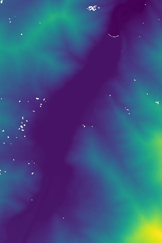
Export to GeoTIFF
The last step is to export the filled DEM to the open standard GeoTIFF file format.
Right click on the filled DEM layer (lake_logan_1m_filled_DEM_final) and select Export. This will bring up the r.out.gdal dialog.
Click on the browse button next to the Name for output raster file option to browse to the directory where you want the geotiff file to be written. Keep the default file format as GTiff (GeoTIFF).
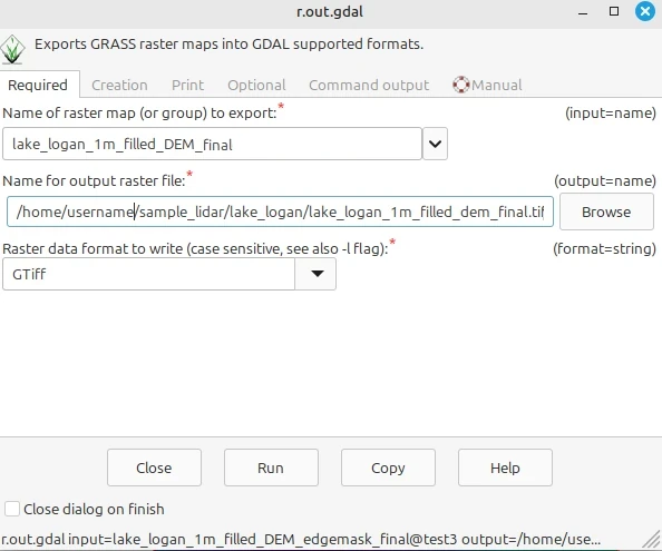
Click on the Creation tab. On this tab you can select the Data type and compression level for the output image. From the Data type drop-down select Float64.
Then go to the Creation option(s) to pass to the output format driver section. The different options for writing out a GeoTIFF raster can be found at the GDAL GeoTiff format description page. Type in “compress=deflate,predictor=3”. Click Run.
r.out.gdal input=lake_logan_1m_filled_DEM_final output=lake_logan_1m_filled_DEM_final.tif format=GTiff type=Float64 createopt="compress=deflate,predictor=3"gs.run_command(
"r.out.gdal",
input="lake_logan_1m_filled_DEM_final",
output="lake_logan_1m_filled_DEM_final.tif",
format="GTiff",
type="Float64",
createopt="compress=deflate,predictor=3",
)
NoteCompression and large datasets
Deflate compression is the most recognized lossless compression for GeoTIFFs. It is supported by other software and is relatively fast for reads. The predictor option allows the deflate compression to be more efficient. You can leave the GeoTIFFs uncompressed, but the file size will be about 4 times larger than the deflate compressed version. This difference adds up as you scale this process up to larger data sets.
For GeoTIFFs larger than 4GB, you will need to use the BIGTIFF=YES option to successfully write an output raster. You may want to also add the num_threads=4 to enable the multi-threaded writing option as well.
Congratulations! You have completed this tutorial!
Resources
Newcomb, D. (2025). A Tutorial on Modeling Water Voids in Airborne LiDAR Point Cloud Data to Hydroflatten Water Surfaces in Digital Elevation Models. Zenodo. https://doi.org/10.5281/zenodo.17121432
The development of this tutorial was in part funded by the US National Science Foundation (NSF), award 2303651.