# Import libraries
import os
import sys
import subprocess
from pathlib import Path

# Find GRASS Python packages
sys.path.append(
  subprocess.check_output(
    ["grass", "--config", "python_path"],
    text=True
    ).strip()
  )

# Import GRASS packages
import grass.script as gs
import grass.jupyter as gj

# Create a temporary folder
import tempfile
temporary = tempfile.TemporaryDirectory()

# Create a project in the temporary directory
gs.create_project(path=temporary.name, name="xy")

# Start GRASS in this project
session = gj.init(Path(temporary.name, "xy"))Earthworks: Terrain Synthesis
earthworks
terrain
raster
intermediate
Learn how to synthesize terrain with r.earthworks.
Learn how to synthesize terrain with r.earthworks [2]. In terrain synthesis, landforms from one terrain are applied to another, creating a hybrid landscape. This technique is used in computer graphics to model landscapes that are challenging to create with procedural noise and erosion simulations [1, 3, 4]. Landforms that are hard to model, for example, can be sampled from real terrain and grafted onto synthetic terrain. In this tutorial, we will use fractal terrain for simplicity’s sake. Our process will be to:
- Setup our environment
- Generate a fractal terrain
- Generate a fractal texture
- Classify landforms in the texture map
- Extract textures for select landforms
- Shift clumps of texture to the same base elevation
- Synthesize the terrain and extracted textures
| Terrain | Texture | Synthesis |
|---|---|---|
 |
 |
 |
NoteComputational notebook
This tutorial can be run as a computational notebook. Learn how to work with notebooks with the tutorial Get started with GRASS & Python in Jupyter Notebooks.
Setup
Project
Start a GRASS session in a new project with a Cartesian (XY) coordinate system.
grass --tmp-project XYInstallation
Install r.earthworks with g.extension.
g.extension extension=r.earthworks# Install extension
gs.run_command("g.extension", extension="r.earthworks")Region
Use g.region to set the extent and resolution of the computational region. Create a region starting at the origin and extending two hundred units north and eight hundred units east. Set the resolution to ten.
g.region n=200 e=800 s=0 w=0 res=1# Set region
gs.run_command("g.region", n=200, e=800, s=0, w=0, res=10)Fractals
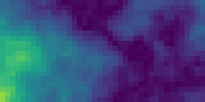
Terrain
Generate a fractal terrain with r.surf.fractal. For reproducible results, set the seed to one. Then use the raster calculator r.mapcalc to take the absolute value of the fractal and divide by a vertical scale factor. Taking the absolute value of the fractal terrain will raise cells with negative elevation values, turning low points into high points and transforming slopes near zero into valleys.
r.surf.fractal output=fractal dimension=2.25 seed=1
r.mapcalc expression="fractal = abs(fractal) / 10"
# Generate fractal surface
gs.run_command(
"r.surf.fractal",
output="fractal",
dimension=2.25,
seed=1
)
gs.mapcalc("fractal = abs(fractal) / 10")
# Visualize
m = gj.Map(width=800)
m.d_rast(map="fractal")
m.d_legend(raster="fractal", at=(5, 95, 1, 3))
m.show()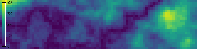
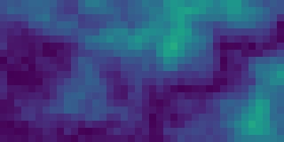
Texture
Repeat this process to generate a fractal texture that will be grafted onto the original terrain. Set a different seed for r.surf.fractal to generate a new fractal raster. If you wish to work with real rather than synthetic elevation data, simply substitute these fractal rasters with digital elevation models for real landscapes.
r.surf.fractal output=texture dimension=2.25 seed=3
r.mapcalc expression="texture = abs(texture) / 10"
# Generate fractal surface
gs.run_command(
"r.surf.fractal",
output="texture",
dimension=2.25,
seed=3
)
gs.mapcalc("texture = abs(texture) / 10")
# Visualize
m = gj.Map(width=800)
m.d_rast(map="texture")
m.d_legend(raster="texture", at=(5, 95, 1, 3))
m.show()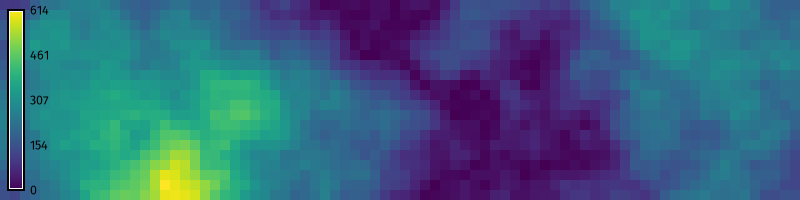
Landforms
Classify the landforms in the fractal texture map with r.geomorphon. Experiment with the search and skip parameters to classify different scales of landforms.
r.geomorphon elevation=texture forms=forms search=9# Classify landforms
gs.run_command(
"r.geomorphon",
elevation="texture",
forms="forms",
search=9
)
# Visualize
m.d_rast(map="forms", flags="n")
m.d_legend(raster="forms", at=(5, 95, 1, 3))
m.show()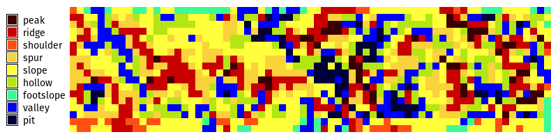
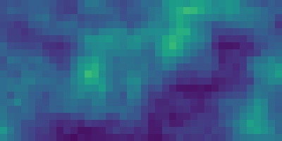
Extraction
Extract textures for the peaks, ridges, shoulders, and spurs with the raster calculator r.mapcalc. Write the map algebra expression ridges = if(forms > 1 && forms < 6, texture, null()). All cells with landforms classes greater than one and less than six will be assigned elevation values from the texture map, while all others will be assigned null values.
r.mapcalc expression="ridges = if(forms > 1 && forms < 6, texture, null())"# Extract ridge texture
gs.mapcalc("ridges = if(forms > 1 && forms < 6, texture, null())")
# Visualize
m.d_rast(map="ridges", flags="n")
m.d_legend(raster="ridges", at=(5, 95, 1, 3))
m.show()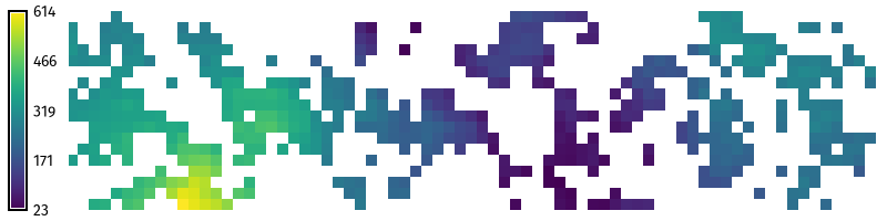
Shift
The map of extracted textures has elevation values that are relative to vertical datum such as mean sea level. Because we will be grafting these textures onto another terrain, we will reset the base elevation for each clump of texture to zero. Find clumps of texture with r.clump. Then use r.stats.zonal to find the minimum value - the base elevation - for each clump. Use the raster calculator r.mapcalc to subtract the minimum value for each clump in the map of extracted textures. This will set the lowest elevation for each clump to zero, so that all clumps share the same base elevation.
r.clump input=ridges output=clumps threshold=0.5
r.stats.zonal base=clumps cover=ridges method=min output=minimum
r.mapcalc expression="ridges = ridges - minimum"
# Find clumps
gs.run_command(
"r.clump",
input="ridges",
output="clumps",
threshold=0.5
)
# Calculate zonal statistics
gs.run_command(
"r.stats.zonal",
base="clumps",
cover="ridges",
method="min",
output="minimum"
)
# Subtract base elevation
gs.mapcalc("ridges = ridges - minimum")
# Visualize
m.d_rast(map="ridges", flags="n")
m.d_legend(raster="ridges", at=(5, 95, 1, 3))
m.show()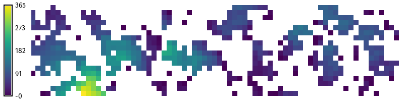
Synthesis
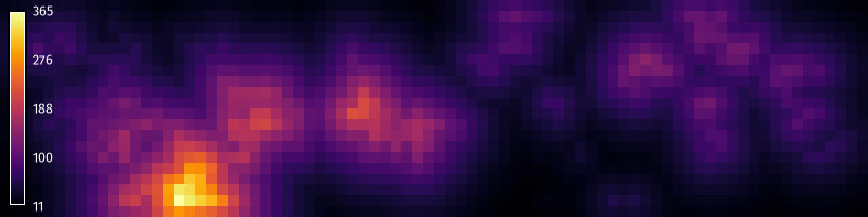
Synthesize the terrain and texture with r.earthworks. Model a fill operation with the extracted textures relative to the fractal terrain. Try setting an exponential rate of decay such as exponential=0.025. Add a volume output to visualize the volumetric change.
r.earthworks elevation=fractal earthworks=synthesis volume=volume mode=relative operation=fill function=exponential raster=ridges exponential=0.025# Synthesize ridges
gs.run_command(
"r.earthworks",
elevation="fractal",
earthworks="synthesis",
volume="volume",
mode="relative",
operation="fill",
function="exponential",
raster="ridges",
exponential=0.025
)
# Visualize
m.d_rast(map="synthesis")
m.d_legend(raster="synthesis", at=(5, 95, 1, 3))
m.show()
# Visualize
gs.run_command("r.colors", map="volume", color="inferno")
m.d_rast(map="volume")
m.d_legend(raster="volume", color="white", at=(5, 95, 1, 3))
m.show()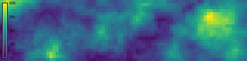
References
[1]
J. Gain, B. Merry, and P. Marais. 2015. Parallel, realistic and controllable terrain synthesis. Computer Graphics Forum 34, 2 (2015), 105–116. https://doi.org/https://doi.org/10.1111/cgf.12545
[2]
Brendan Harmon, Anna Petrasova, and Vaclav Petras. 2026. r.earthworks: A GRASS tool for terrain modeling. Journal of Open Source Software 11, 118 (2026), 9270. https://doi.org/10.21105/joss.09270
[3]
F. P. Tasse, J. Gain, and P. Marais. 2012. Enhanced texture-based terrain synthesis on graphics hardware. Computer Graphics Forum 31, 6 (2012), 1959–1972. https://doi.org/https://doi.org/10.1111/j.1467-8659.2012.03076.x
[4]
Howard Zhou, Jie Sun, Greg Turk, and James M. Rehg. 2007. Terrain synthesis from digital elevation models. IEEE Transactions on Visualization and Computer Graphics 13, 4 (2007), 834–848. https://doi.org/10.1109/TVCG.2007.1027