Earthworks: Gully Modeling

Model gullies using relative cut operations with r.earthworks.

Gullies

Learn the how to model gullies using relative cut operations with r.earthworks. This tutorial introduces more features of r.earthworks including vector line input, relative operations, exponential functions, and volumetric change calculations. While absolute operations calculate cut and fill based on a vertical datum of zero and can be used to model features at a given elevation, relative operations calculate cut and fill relative to the existing topography and can be used to model features that follow the existing terrain.

Use a relative earthworking operation with an exponential function to carve deep gullies into a landscape. In this tutorial all of the data will be created procedurally including the terrain and the streams. Start by generating fractal terrain. Then model flow accumulation through the fractal terrain and extract its stream network. Finally use the vector map of streams as input for a relative cut operation to transform valleys into deep gullies. This tutorial covers:

• Terrain generation
• Flow accumulation
• Stream extraction
• Relative earthworks

For a simulation based approach to modeling gullies, try the landscape evolution model r.sim.terrain instead.

Computational notebook

This tutorial can be run as a computational notebook. Learn how to work with notebooks in the tutorial Get started with GRASS & Python in Jupyter Notebooks.

Setup

Project

Start a GRASS session in a new project with a Cartesian (XY) coordinate system.

Command line

grass --tmp-project XY

Python

# Import libraries
import os
import sys
import subprocess
from pathlib import Path

# Find GRASS Python packages
sys.path.append(
  subprocess.check_output(
    ["grass", "--config", "python_path"],
    text=True
    ).strip()
  )

# Import GRASS packages
import grass.script as gs
import grass.jupyter as gj

# Create a temporary folder
import tempfile
temporary = tempfile.TemporaryDirectory()

# Create a project in the temporary directory
gs.create_project(path=temporary.name, name="xy")

# Start GRASS in this project
session = gj.init(Path(temporary.name, "xy"))

Installation

Install r.earthworks and r.stream.order with g.extension.

Command line

g.extension extension=r.earthworks
g.extension extension=r.stream.order

Python

# Install extension
gs.run_command("g.extension", extension="r.earthworks")
gs.run_command("g.extension", extension="r.stream.order")

Region

Use g.region to set the extent and resolution of the computational region. Create a region starting at the origin and extending two hundred units north and eight hundred units east.

Command line

g.region n=200 e=800 s=0 w=0 res=1

Python

# Set region
gs.run_command("g.region", n=200, e=800, s=0, w=0, res=1)

Fractal Terrain

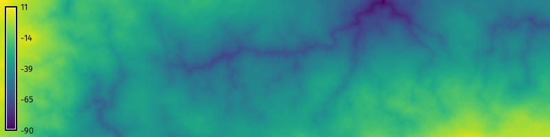
Generate a fractal terrain with r.surf.fractal. Running this tool without setting a seed will generate random results each run. For reproducible results set a seed. Then use the raster calculator r.mapcalc to scale it vertically so that the mountains are not too high.

Command line

r.surf.fractal output=fractal seed=1
r.mapcalc expression="fractal = fractal / 10" --overwrite
r.stream.extract elevation=fractal accumulation=accumulation threshold=1000 stream_vector=streams

Python

# Generate fractal surface
gs.run_command(
    "r.surf.fractal",
    output="fractal",
    seed=1
    )
gs.mapcalc("fractal = fractal / 10")

# Visualize
m = gj.Map(width=800)
m.d_rast(map="fractal")
m.d_legend(raster="fractal", at=(5, 95, 1, 3))
m.show()

Fractal terrain

Stream Network

Model a stream network for the fractal landscape. First use r.watershed to compute flow accumulation through the landscape. Then use r.stream.extract to extract a vector stream network. Try different threshold values to experiment with the minimum flow accumulation required for streams. Calculate the hierarchy of the stream network with r.stream.order. Use map algebra with r.mapcalc to estimate the depth of gullies by scaling the resulting Strahler stream order raster map. Use a negative scaling factor.

Command line

r.watershed elevation=fractal accumulation=accumulation -b
r.stream.extract elevation=fractal accumulation=accumulation threshold=1000 stream_vector=streams stream_raster=streams direction=direction
r.stream.order elevation=fractal accumulation=accumulation stream_rast=streams stream_vect=streams direction=direction strahler=strahler --overwrite
r.mapcalc expression="gullies = strahler * -5"

Python

# Compute flow accumulation
gs.run_command(
    "r.watershed",
    elevation="fractal",
    accumulation="accumulation",
    flags='b'
    )

# Extract stream network
gs.run_command("r.stream.extract",
    elevation="fractal",
    accumulation="accumulation",
    threshold=1000,
    stream_vector="streams",
    stream_raster="streams",
    direction="direction"
    )

# Calculate stream order
gs.run_command("r.stream.order",
    elevation="fractal",
    accumulation="accumulation",
    stream_rast="streams",
    stream_vect="streams",
    direction="direction",
    strahler="strahler"
    )

# Scale raster
gs.mapcalc("gullies = strahler * -5")

# Visualize
m = gj.Map(width=800)
m.d_rast(map="fractal")
m.d_vect(map="streams", type="line", color="white", width_column="strahler")
m.d_legend(raster="fractal", at=(5, 95, 1, 3))
m.show()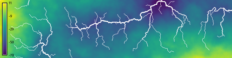

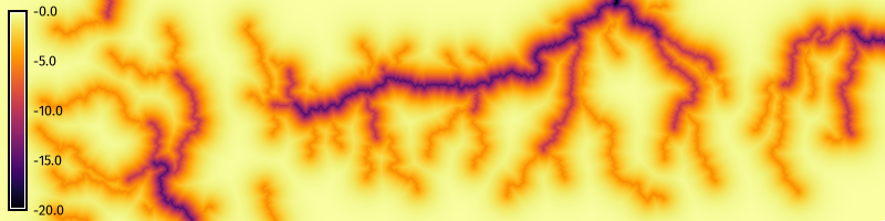
Stream network

Relative Cut Operation

Use r.earthworks to cut deep gullies into the stream channels. Use the exponential growth and decay function \(z = z_0 e^{-\lambda \sqrt{\Delta x^2 + \Delta y^2}}\) to model the steep slopes of the gullies. Set mode to relative, operation to cut, function to exponential, raster to the raster map of gullies, and rate \(\lambda\) to a value such as 0.1. Save an output volume raster to visualize volumetric change. This may take a minute to run. For faster results, try setting a lower resolution with g.region.

Command line

r.earthworks elevation=fractal earthworks=gullies volume=volume mode=relative operation=cut function=exponential raster=gullies rate=0.1 --overwrite
r.colors map=volume color=inferno

Python

# Model gullies
gs.run_command(
    "r.earthworks",
    elevation="fractal",
    earthworks="gullies",
    volume="volume",
    mode="relative",
    operation="cut",
    function="exponential",
    raster="gullies",
    rate=0.1
    )
gs.run_command("r.colors", map="volume", color="inferno")

# Visualize
m = gj.Map(width=800)
m.d_rast(map="gullies")
m.d_legend(raster="gullies", at=(5, 95, 1, 3))
m.show()

# Visualize volume
m = gj.Map(width=800)
m.d_rast(map="volume")
m.d_legend(raster="volume", at=(5, 95, 1, 3))
m.show()

Gullies

Volumetric change