# Import libraries
import os
import sys
import subprocess
from pathlib import Path

# Find GRASS Python packages
sys.path.append(
  subprocess.check_output(
    ["grass", "--config", "python_path"],
    text=True
    ).strip()
  )

# Import GRASS packages
import grass.script as gs
import grass.jupyter as gj

# Create a temporary folder
import tempfile
temporary = tempfile.TemporaryDirectory()

# Create a project in the temporary directory
gs.create_project(path=temporary.name, name="xy")

# Start GRASS in this project
session = gj.init(Path(temporary.name, "xy"))Earthworks: Basics
earthworks
terrain
raster
beginner
Learn the basics of terrain modeling with r.earthworks.
Learn the basics of terrain modeling with r.earthworks [1]. This tool uses cut and fill operations to transform topography. Cut operations subtract from a topographic surface, while fill operations add to the topography. Transformations are based on proposed local topographic extrema, i.e. high points and low points. These extrema can be set with coordinates, rasters, vector points, or vector lines. In GRASS raster and vector data can be drawn with the raster digitizer and vector digitizer. Transformations are a function of the existing elevation, change in vertical distance, and change in slope over horizontal distance. Vertical distance is calculated as the difference between proposed local extrema and a topographic datum, while change in slope is a function of growth and decay applied to horizontal change in distance. This tutorial covers:
- Cut operations
- Fill operations
- Cut & fill operations
- Random operations
NoteComputational notebook
This tutorial can be run as a computational notebook. Learn how to work with notebooks with the tutorial Get started with GRASS & Python in Jupyter Notebooks.
Setup
Project
Start a GRASS session in a new project with a Cartesian (XY) coordinate system.
grass --tmp-project XYInstallation
Install r.earthworks with g.extension.
g.extension extension=r.earthworks# Install extension
gs.run_command("g.extension", extension="r.earthworks")Region
Use g.region to set the extent and resolution of the computational region. Create a region starting at the origin and extending two hundred units north and eight hundred units east. Use the raster calculator r.mapcalc to generate a flat terrain with an constant elevation of zero.
g.region n=200 e=800 s=0 w=0 res=1
r.mapcalc expression="elevation = 0"
# Set region
gs.run_command("g.region", n=200, e=800, s=0, w=0, res=1)
# Generate base elevation
gs.mapcalc("elevation = 0")
Fill Operations
Use a fill operation to model a peak from a set of x- and y-coordinates with r.earthworks. These coordinates represents a local topographic maxima, i.e. a high point. The algorithm will fill locally up to that point, then the slopes will fall off at a given rate of decay. Set coordinates to a pair of x- and y-coordinates. Use the z parameter to set a z-coordinate for the top of the peak. Optionally use the flat parameter to create a plateau at the top of the peak. Using the default linear growth and decay function \(z = z_0 - r \sqrt{\Delta x^2 + \Delta y^2}\), set the linear slope parameter to 0.5 to model a 50 percent slope.
r.earthworks elevation=elevation earthworks=peak operation=fill function=linear linear=0.5 coordinates=400,100 z=25 flat=25# Model earthworks
gs.run_command(
"r.earthworks",
elevation="elevation",
earthworks="peak",
operation="fill",
function="linear",
linear=0.5,
coordinates=[400, 100],
z=25,
flat=25
)
# Visualize
m = gj.Map(width=800)
m.d_rast(map="peak")
m.d_legend(raster="peak", color="white", at=(5, 95, 1, 3))
m.show()
Cut Operations
Use a cut operation to model a pit from a set of x- and y-coordinates with r.earthworks. Set a z-coordinate for the bottom of the pit. These coordinates represents a local topographic minima, i.e. a low point. The algorithm will cut locally down to that point, then the slopes will climb at a given rate of growth.
r.earthworks elevation=elevation earthworks=pit operation=cut function=linear linear=0.5 coordinates=400,100 z=-25 flat=25# Model earthworks
gs.run_command(
"r.earthworks",
elevation="elevation",
earthworks="pit",
operation="cut",
function="linear",
linear=0.5,
coordinates=[400, 100],
z=-25,
flat=25
)
# Visualize
m = gj.Map(width=800)
m.d_rast(map="pit")
m.d_legend(raster="pit", color="black", at=(5, 95, 1, 3))
m.show()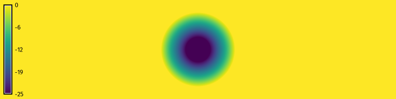
Cut & Fill Operations
Use cut and fill operations to model a pit and a peak from two sets of x- and y-coordinates with r.earthworks. Set a z-coordinate for the bottom of the pit and another z-coordinate for the top of the peak.
r.earthworks elevation=elevation earthworks=pit_and_peak operation=cutfill function=linear linear=0.5 coordinates=350,100,450,100 z=-25,25 flat=25# Model earthworks
gs.run_command(
"r.earthworks",
elevation="elevation",
earthworks="pit_and_peak",
operation="cutfill",
function="linear",
linear=0.5,
coordinates=[350, 100, 450, 100],
z=[-25, 25],
flat=25
)
# Visualize
m = gj.Map(width=800)
m.d_rast(map="pit_and_peak")
m.d_legend(raster="pit_and_peak", color="black", at=(5, 95, 1, 3))
m.show()
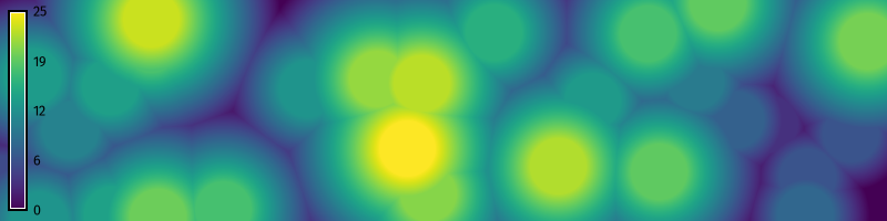
Random Operations
Randomness
Model a set of random peaks by generating a random surface, sampling random points, and then filling on those points. First generate a random surface with r.surf.random. Set a seed for reproducible results or set flags="s" for a random seed. Then randomly sample 50 cells from the random surface r.random. Use a fill operation to model random peaks with r.earthworks. Set input raster to the random cells.
r.surf.random out=surface min=0 max=25 seed=2
r.random input=surface npoints=50 raster=random seed=7
r.earthworks elevation=elevation earthworks=earthworks operation=fill raster=random function=linear linear=0.25 flat=25
# Generate random surface
gs.run_command("r.surf.random", out="surface", min=0, max=25, seed=2)
# Sample random points
gs.run_command(
"r.random",
input="surface",
npoints=50,
raster="random",
seed=7
)
# Model earthworks
gs.run_command(
"r.earthworks",
elevation="elevation",
earthworks="earthworks",
operation="fill",
raster="random",
function="linear",
linear=0.25,
flat=25
)
# Visualize
m = gj.Map(width=800)
m.d_rast(map="earthworks")
m.d_legend(raster="earthworks", digits=0, at=(5, 95, 1, 3))
m.show()
Visualization
Compute contours for earthworks with r.contour.
r.contour input=earthworks output=contours step=2# Derive contours
gs.run_command("r.contour", input="earthworks", output="contours", step=2)
# Visualize Contours
m = gj.Map(width=800)
m.d_vect(map="contours")
m.show()
References
[1]
Brendan Harmon, Anna Petrasova, and Vaclav Petras. 2026. r.earthworks: A GRASS tool for terrain modeling. Journal of Open Source Software 11, 118 (2026), 9270. https://doi.org/10.21105/joss.09270